Post Result

Toolbar

• Show Workpieces Only - Shows only the workpieces in the Post view.
• Show Upper/Lower Dies Only - Shows only the dies in the Post view.
• Show Upper Dies Only - Shows only the upper dies in the Post view.
• Show Lower Dies Only - Shows only the lower dies in the Post view.
• Show Workpieces/Upper Dies Only - Shows only the workpieces and upper dies in the Post view.
• Show Workpieces/Lower Dies Only - Shows only the workpieces and lower dies in the Post view.
• Show All - Shows all shapes in the Post view.
• Reset to Focus on Workpieces - Resets the Post view and renders the workpieces as face / (face + outline) / (face + elements).
• Reset to Focus on Dies - Resets the Post view and renders the dies as face / (face + outline) / (face + elements).
• Reset all - Resets the Post view and renders all shapes as face / (face + outline) / (face + elements).

Mechanical

Lists the result items related to the mechanical properties among the analysis results.

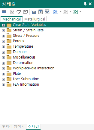
Clear State Variables

Displays each shape in the color assigned to it.

Strain / Strain Rate

Results related to strain \(\varepsilon\) and strain rate \(\dot{\varepsilon}\)

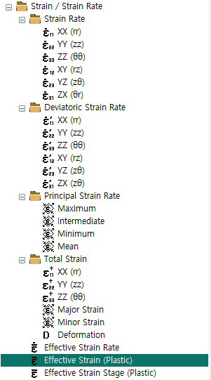
• Effective Strain Rate - Shows the effective strain rate \(\dot{\bar{\varepsilon}}\).

\[ \begin{aligned} \dot{\bar{\varepsilon}} &= \sqrt{\frac{2}{3} \sum_{i=1}^{3}\sum_{j=1}^{3} \dot\varepsilon'_{ij} \dot\varepsilon'_{ij} } \\ &= \frac{\sqrt{2}}{3}\left[ \left( \dot{\varepsilon}_{xx} - \dot{\varepsilon}_{yy} \right)^2 + \left( \dot{\varepsilon}_{yy} - \dot{\varepsilon}_{zz} \right)^2 + \left( \dot{\varepsilon}_{zz} - \dot{\varepsilon}_{xx} \right)^2 +6\left({ \dot{\varepsilon}_{xy}}^2 + {\dot{\varepsilon}_{yz}}^2 + {\dot{\varepsilon}_{zx}}^2 \right) \right]^{\frac{1}{2}} \end{aligned} \]

• Effective Strain (Plastic) - Shows the effective strain (plastic) \(\bar{\varepsilon}_p\).

\[ \begin{aligned} {\bar{\varepsilon}} &= \sqrt{\frac{2}{3} \sum_{i=1}^{3}\sum_{j=1}^{3} \varepsilon'_{ij} \varepsilon'_{ij} } \\ &= \frac{\sqrt{2}}{3}\left[ \left( {\varepsilon}_{xx} - {\varepsilon}_{yy} \right)^2 + \left( {\varepsilon}_{yy} - {\varepsilon}_{zz} \right)^2 + \left( {\varepsilon}_{zz} - {\varepsilon}_{xx} \right)^2 +6\left({ {\varepsilon}_{xy}}^2 + {{\varepsilon}_{yz}}^2 + {{\varepsilon}_{zx}}^2 \right) \right]^{\frac{1}{2}} \end{aligned} \]

• Effective Strain Stage (Plastic) - Shows the effective strain (plastic) \(\bar{\varepsilon}_p\) accumulated in the corresponding stage.

Strain Rate

Shows the components \(\dot{\varepsilon}_{ij}\) of the strain rate tensor.
The symmetric part of the velocity gradient tensor \(\frac{\partial v_i}{\partial x_j}\),

\[ \dot{\varepsilon}_{ij} =\frac{1}{2} \left( \frac{\partial v_i}{\partial x_j} + \frac{\partial v_j}{\partial x_i} \right) \]

is called the strain rate. Here \(v_i\) is a velocity component and \(x_i\) is a coordinate direction.

Deviatoric Strain Rate

Shows the components \(\dot{\varepsilon}'_{ij}\) of the deviatoric strain rate tensor.

\[ \dot{\varepsilon}'_{ij} = \dot{\varepsilon}_{ij} - \frac{1}{3}\delta_{ij}\dot{\varepsilon}_{kk} \]

Here \(\delta_{ij}\) is the Kronecker delta.

Principal Strain Rate

Shows the principal strain rates and the mean strain rate.
The strain rate is a second-order tensor quantity. From the following eigenvalue problem for the strain rate tensor \(\dot{\varepsilon}_{ij}\),

\[ \sum_{j=1}^{3} \dot{\varepsilon}_{ij}n_j = \dot{\varepsilon}n_i \text{ or } \begin{pmatrix} \dot{\varepsilon}_{xx} & \dot{\varepsilon}_{xy} & \dot{\varepsilon}_{xz} \\ \dot{\varepsilon}_{yx} & \dot{\varepsilon}_{yy} & \dot{\varepsilon}_{yz} \\ \dot{\varepsilon}_{zx} & \dot{\varepsilon}_{zy} & \dot{\varepsilon}_{zz} \end{pmatrix} \begin{pmatrix} n_{x} \\ n_{y} \\ n_{z} \end{pmatrix} = \dot{\varepsilon} \begin{pmatrix} n_{x} \\ n_{y} \\ n_{z} \end{pmatrix} \]

three principal strain rates \(\dot{\varepsilon}_{1}\), \(\dot{\varepsilon}_{2}\), \(\dot{\varepsilon}_{3}\) are defined. The mean strain rate \(\dot{\varepsilon}\) is the average of the computed principal strain rates.

Total Strain

Shows the normal strain components \(\varepsilon_{ii}\), the maximum strain \(\varepsilon_{1}\) and the minimum strain \(\varepsilon_{3}\).

Stress / Pressure

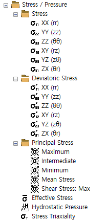
Stress

Shows the components \(\sigma_{ij}\) of the stress tensor.

\[ \sigma_{ij} = \lim_{\Delta A_i \to 0 } \frac{\Delta F_j}{\Delta A_i } \]

Here \(A_i\) is an infinitesimal area on the surface defined by \(\mathbf{n} = \mathbf{e}_i\). Expressed in matrix form, the stress components are as follows.

\[ \begin{pmatrix} \sigma_{11} & \sigma_{12} & \sigma_{13}\\ \sigma_{21} & \sigma_{22} & \sigma_{23}\\ \sigma_{31} & \sigma_{32} & \sigma_{33} \end{pmatrix} \text{ or } \begin{pmatrix} \sigma_{xx} & \sigma_{xy} & \sigma_{xz}\\ \sigma_{yx} & \sigma_{yy} & \sigma_{yz}\\ \sigma_{zx} & \sigma_{zy} & \sigma_{zz} \end{pmatrix} \]

Deviatoric Stress

Shows the deviatoric stress tensor \({\sigma_{ij}}'\).

\[ {\sigma_{ij}}' = \sigma_{ij} - \frac{1}{3} \delta_{ij}\sigma_{kk} \]

Principal Stress

Shows the principal stresses \( \sigma_1, \sigma_2, \sigma_3 \), the mean stress \(\sigma_\text{m}\) and the maximum shear stress \(\tau_\text{max}\).

On the principal stress axes the shear stress components are zero, and the direction of the principal stress \(\mathbf{n}\) and the magnitude of the principal stress \(\sigma_N\) must satisfy the following relation.

\[ \begin{pmatrix} \sigma_{xx} & \sigma_{xy} & \sigma_{xz}\\ \sigma_{yx} & \sigma_{yy} & \sigma_{yz}\\ \sigma_{zx} & \sigma_{zy} & \sigma_{zz} \end{pmatrix} \begin{pmatrix} n_x \\ n_y \\ n_z \end{pmatrix} = \sigma_N \begin{pmatrix} n_x \\ n_y \\ n_z \end{pmatrix} \]

This equation is a homogeneous linear equation and an eigenvalue problem. For this eigenvalue problem to have a meaningful solution, the following characteristic equation must be satisfied.

\[ \left| \sigma_{ij} - \sigma_N \delta_{ij} \right| = 0 \]

This characteristic equation implies that the system is made indeterminate so that it has infinitely many solutions; that is, the linear equations are made linearly dependent. Rearranging this condition yields the following cubic algebraic equation. The solutions for \( \sigma_N \) are called the principal stresses.

\[ \sigma^3_N -I_1\sigma^2_N+I_2\sigma_N-I_3 = 0 \]

Here \(I_1\), \(I_2\) and \(I_3\) are defined as follows.

\[ \begin{aligned} I_1 &= \sigma_{xx}+ \sigma_{yy}+\sigma_{zz} \\ I_2 &= \sigma_{xx}\sigma_{yy} + \sigma_{yy}\sigma_{zz} + \sigma_{zz}\sigma_{xx} - {\sigma_{xy}}^2 - {\sigma_{yz}}^2 - {\sigma_{zx}}^2 \\ I_3 &= \sigma_{xx}\sigma_{yy}\sigma_{zz}+2\sigma_{xy}\sigma_{yz}\sigma_{zx}-\sigma_{xx}{\sigma_{yz}}^2-\sigma_{yy}{\sigma_{zx}}^2-\sigma_{zz}{\sigma_{xy}}^2 \end{aligned} \]

• Effective Stress - Shows the effective stress \(\bar{\sigma}\).

\[ \begin{aligned} \bar{\sigma} &= \sqrt{3J_2} \\ &=\sqrt{\frac{2}{3} \sum_{i=1}^{3}\sum_{j=1}^{3} \sigma'_{ij} \sigma'_{ij} } \\ &= \sqrt{ \frac{1}{2} \left[ \left( {\sigma}_{xx} - {\sigma}_{yy} \right)^2 + \left( {\sigma}_{yy} - {\sigma}_{zz} \right)^2 + \left( {\sigma}_{zz} - {\sigma}_{xx} \right)^2 +6{ {\sigma}_{xy}}^2 + 6{{\sigma}_{yz}}^2 + 6{{\sigma}_{zx}}^2 \right] } \\ &= \sqrt{ \frac{1}{2} \left[ \left( {\sigma}_{1} - {\sigma}_{2} \right)^2 + \left( {\sigma}_{2} - {\sigma}_{3} \right)^2 + \left( {\sigma}_{3} - {\sigma}_{1} \right)^2 \right] } \end{aligned} \]

• Hydrostatic Pressure - Shows the hydrostatic pressure \(p\).

\[ p = -\sigma_\text{m} \]

Here \(\sigma_\text{m}\) is the mean stress.

• Stress Triaxiality - Shows the stress triaxiality \(\eta\).

\[ \eta = \frac{\sigma_\text{m}}{\bar\sigma} \]

Porous

Shows the powder forming analysis results.

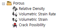
• Relative Density - Shows the relative density. The relative density is the density of the porous material divided by the density of a theoretical non-porous material of the same volume.
• Volumetric Strain Rate - Shows the volumetric strain rate. The volumetric strain rate is the rate of change of the volumetric strain with respect to time.
• Volumetric Strain - Shows the volumetric strain. The volumetric strain is the ratio of the volume change that occurs while a porous material is compressed or expanded.
• Crack Possibility - Shows the fracture possibility.

Temperature

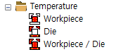
• Workpiece - Shows the temperature distribution of the workpiece.
• Die - Shows the temperature distribution of the die.
• Workpiece / Die - Shows the temperature distributions of the workpiece and the die.

Damage

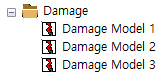
• Damage Model 1 - Shows the distribution of the model stored in damage 1.
• Damage Model 2 - Shows the distribution of the model stored in damage 2.
• Damage Model 3 - Shows the distribution of the model stored in damage 3.

Miscellaneous

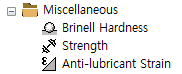
• Brinell Hardness - Shows the Brinell hardness.
• Strength - Shows the strength.
• Anti-lubricant Strain - Shows the lubricant damage ratio.

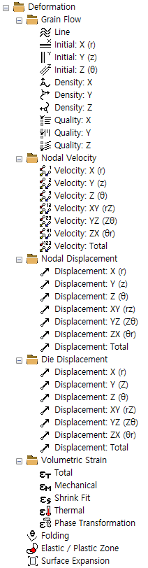
Deformation

Shows the items related to deformation.

Grain Flow

The grain flow line is expressed as a function of the initial coordinates. This function is a vector function; that is, at a single point it has two or more values (two in two dimensions, three in three dimensions). Writing this function as

\[ \phi_i = \phi_i\left(x_p\right) \]

we call it the grain flow function. The curves or surfaces on which each component of this vector function takes a constant value are directly or indirectly connected to the grain flow lines; the direction of its gradient is perpendicular to the grain flow lines, and its magnitude represents the density of the grain flow lines. Accordingly, the gradient of the grain flow function is defined as the grain flow density. The gradient of the grain flow density is a second-order tensor, that is the grain flow tensor, from which the overlapping index can be defined.

\[ \begin{aligned} g_i &= \nabla\phi_i \\ G^i_{pq} &= \frac{\partial^2\phi_i}{\partial x_p\partial x_q} \\ \bar{G^i} &= \sqrt{\frac{2}{3}{G^i_{pq}}'{G^i_{pq}}'} \end{aligned} \]

Here \(g_i\) is the grain flow density, \(G^i_{pq}\) is the grain flow tensor, and \(\bar{G^i}\) is the overlapping index.

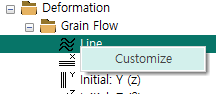
• Line - Shows the grain flow lines. Right-clicking this item brings up a Context menu. Clicking the Customize item brings up the Grain flow line settings dialog.
  

• Initial - Shows the grain flow function (initial coordinates) in the X/Y/Z directions.

• Density - Shows the grain flow density in the X/Y/Z directions.
• Overlapping Index - Shows the overlapping index in the X/Y/Z directions.

Nodal Velocity

Shows the components and the magnitude of the velocity field.

Die Displacement

Shows the components and the magnitude of the die displacement.

Vouemetric Strain

Shows the volumetric strain due to total / mechanical / shrink fitting / temperature / phase transformation.

• Folding - Shows folding.
• Elastic / Plastic Zone - Shows the elastic/plastic zones.
• Surface Expansion - Shows the surface expansion ratio.

Workpiece-die interaction

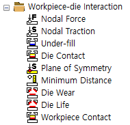
• Nodal Force - Shows the surface force distribution.
• Nodal Traction - Shows the traction vector distribution.
• Under-fill - Shows the under-fill distribution.
• Die Contact - Shows the die contact distribution.
• Plane of Symmetry - Shows the planes of symmetry.
• Minimum Distance - Shows the minimum distance.
• Die Wear - Shows the die wear distribution.
• Die Life - Shows the die life distribution.
• Workpiece Contact - For a multi-body analysis, shows the workpiece-to-workpiece contact distribution.

Plate

Thickness

Shows the thickness in the X/Y/Z directions and along the shortest distance.

Thining

Shows the distribution of the thickness reduction ratio relative to the initial thickness.

• FLD - Shows the forming limit distribution.

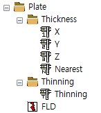
User Subroutine

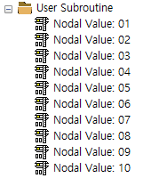
Shows the values stored when the simulation is run using Dll_UserRoutine.dll. Up to 10 values can be stored.

FEA Information

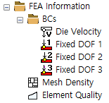
BCs

• Die Velocity - Shows the die velocity distribution over the region where the workpiece and the die are in contact.

• Fixed DOF - Shows the points at which degrees of freedom 1/2/3 are constrained.

• Mesh Density - Shows the mesh density distribution.

• Element Quality - Shows the element quality distribution.

Metallugical

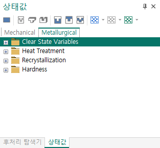
Heat Treatment

The result distributions that appear for a heat treatment analysis.

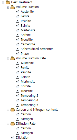
Volume Fraction

Shows the distribution of the Austenite/Ferrite/Pearlite/Bainite/Martensite/Sorbite/Troosite/Cementite/Spheroidized cementite phases.

Volume Fraction Rate

Shows the distribution of the rate of change of the Austenite/Ferrite/Pearlite/Bainite/Martensite/Sorbite/Troosite/Cementite/Spheroidized cementite phases.

Carbon and Nitrogen contents

Shows the distribution of the content of Carbon/Nitrogen.

Diffusion Rate

Shows the distribution of the diffusion rate of Carbon/Nitrogen.

Recrystallization

The result distributions that appear for a recrystallization analysis.

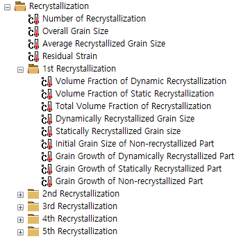
• Number of Recerystallization - Shows the distribution of the number of recrystallizations.
• Overall Grain Size - Shows the distribution of the overall grain size.
• Average Recerstallizaed Grain Size - Shows the distribution of the average recrystallized grain size.
• Residual Strain - Shows the distribution of the residual strain.

1/2/3/4/5th Recerystallization

• Volume Fraction of Dynamic Recrystallization - Shows the distribution of the dynamic recrystallization fraction.
• Volume Fraction of Static Recrystallization - Shows the distribution of the static recrystallization fraction.
• Total Volume Fraction of Recrystallization - Shows the distribution of the total recrystallization fraction.
• Dynamically Recrystallized Grain Size - Shows the distribution of the grain size due to dynamic recrystallization.
• Statically Recrystallized Grain size - Shows the distribution of the grain size due to static recrystallization.
• Initial Grain Size of Non-recrystallized Part - Shows the distribution of the initial grain size of the non-recrystallized part.
• Grain Growth of Dynamically Recrystallized Part - Shows the distribution of the grain growth of the dynamically recrystallized part.
• Grain Growth of Statically Recrystallized Part - Shows the distribution of the grain growth of the statically recrystallized part.
• Grain Growth of Non-recrystallized Part - Shows the distribution of the grain growth of the non-recrystallized part.

Hardness

• Brinell - Shows the Brinell hardness distribution.