A. Tensor Quantities and Index Notation¶

A.1 Mechanical Quantities and Tensor Quantities¶

The mechanical quantities that are the principal objects of analysis in mechanics—namely displacement, strain, stress, temperature, and so on—generally vary from one material point to another. Since the location of each material point is determined or defined by its coordinates, the mechanical quantities of a continuum are functions of coordinates, or of position.

Coordinates express the relative position of a material point with respect to a reference coordinate system. Consequently, even when the same point is expressed, its coordinate values differ depending on the form and location of the reference coordinate system. Vector quantities such as force and displacement, on the other hand, possess both magnitude and direction. Among the ways of expressing these properties of a vector, the most general and effective is to express them as components with respect to a reference coordinate system. The same holds for stress. The definition of a mechanical quantity is therefore inseparable from the coordinate system.

The coordinate systems most widely used in mechanics are orthogonal coordinate systems, of which the rectangular (Cartesian) coordinate system, the cylindrical coordinate system, and the spherical coordinate system are representative examples. Special coordinate systems may also be used when convenient. In most cases, however, the rectangular coordinate system is used; in particular, when the finite element method is adopted as the solution technique, all problems can be solved in a rectangular coordinate system. Rectangular coordinate systems having different orientations are regarded as different coordinate systems. The coordinates of the same point and the mechanical quantities at that point take different numerical values when viewed in different coordinate systems, and they obey a fixed transformation law defined between the two coordinate systems. It should be emphasized that, although the coordinate values expressing an object or material point and the numerical values of the mechanical quantities are expressed differently depending on the coordinate system, the geometric shape of the object and the physical meaning of the mechanical quantities remain unchanged.

Example A.1

Figure A.1 shows two rectangular coordinate systems, the \(x-y\) coordinate system and the \(x'-y'\) coordinate system. The \(x'-y'\) coordinate system is placed in the orientation obtained by rotating the \(x-y\) coordinate system counterclockwise by \(\theta = 30^\circ\). When the \(x-y\) coordinate values of point \(P\) are \((2, 4)\), find the \(x'-y'\) coordinate values of point \(P\).

Solution

The \((x', y')\) coordinates of point \(P\) are calculated as \((2+\sqrt{3}, -1+2\sqrt{3})\). The background of this calculation is detailed in Example 2.2. The absolute values, i.e., the magnitudes, of the two vectors are equal at \(2\sqrt{5}\), and their directions are also equal when the orientation of the coordinate systems is taken into account, since \(\phi - \phi' = \tan^{-1}(4/2) - \tan^{-1}((-1+2\sqrt{3})/(2+\sqrt{3})) = 30^\circ\).

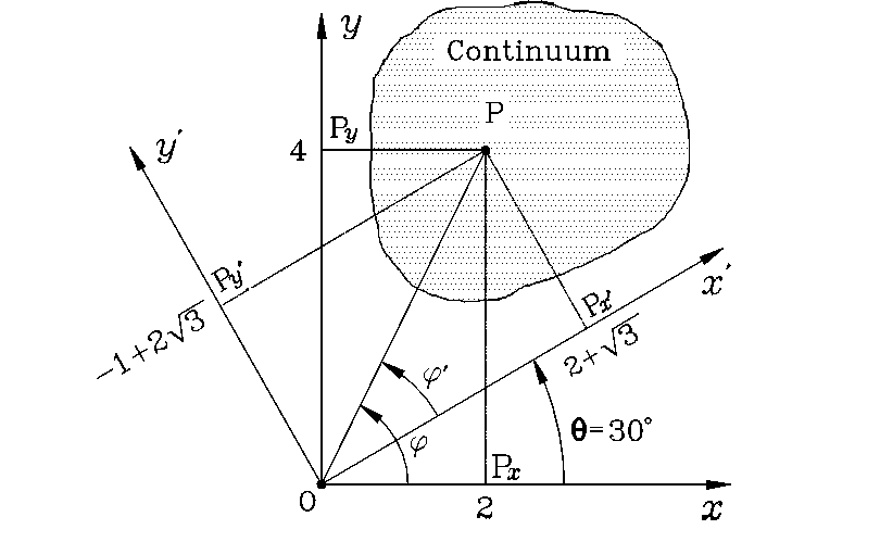
Figure A 1 Coordinate systems and coordinates

As stated above, although a mechanical quantity at a given point may be expressed by different numerical values depending on the coordinate system, the physical meaning of that mechanical quantity is the same. Every mechanical quantity obeys a special form of transformation law according to the characteristics of the group to which it belongs. Mechanical quantities are classified—based on the transformation law they obey—into scalar quantities, vector quantities, dyadic quantities, and so on. Let us deepen our understanding of each quantity through examples.

Let us first explain scalar quantities using temperature as an example. Since the temperature at each material point of a body may differ, temperature is a function of position (for example, in a two-dimensional problem, \(T = T(x,y)\)). In Figure A.1, when the temperature at point \(P\) is 150°C, the temperature is expressed with respect to the \(x-y\) coordinate system and the \(x'-y'\) coordinate system as \(T(2,4) = \text{150°C}\) and \(T'(2+\sqrt{3}, -1+2\sqrt{3}) = \text{150°C}\), respectively. That is,

\[ T'(2+\sqrt{3}, -1+2\sqrt{3}) = T(2,4) = \text{150°C} \tag{A.1} \]

Here \(T'\) denotes the temperature from the viewpoint of the \(x'-y'\) coordinate system. From Equation (A.1) it can be seen that the numerical value of 150 does not change even when the coordinate system is changed. It should be emphasized that the temperature at a point is expressed by the same value even when the coordinate system differs. Mechanical quantities falling into this category are called scalar quantities.

Displacement, force, and the like are different from temperature. The same displacement is expressed by different components depending on the coordinate system. This is because vector quantities, including displacement, possess not only magnitude but also direction. The explanation is given using the position vector as an example. As shown in Figure A.1, the position vector expressed as \((4, 4)\) in the \(x-y\) coordinate system is expressed as \((2+\sqrt{3}, -1+2\sqrt{3})\) in the \(x'-y'\) coordinate system. These two vectors satisfy the following relation.

\[ \begin{bmatrix} 2+\sqrt{3} \\ -1+2\sqrt{3} \end{bmatrix} = \begin{bmatrix} \cos\theta & \sin\theta \\ -\sin\theta & \cos\theta \end{bmatrix} \begin{bmatrix} 2 \\ 4 \end{bmatrix} \tag{A.2} \]

Here

\[ \mathbf{T} = \begin{bmatrix} \cos\theta & \sin\theta \\ -\sin\theta & \cos\theta \end{bmatrix} \tag{A.3} \]

is the transformation matrix, which is an orthonormal matrix. The above relation can be used for the coordinate transformation of any vector quantity. Therefore, in general, if the components of a vector with respect to one coordinate system are known, its components with respect to another coordinate system can be obtained from the transformation relation of Equation (A.2).

Example A.2

Derive the general form of Equation (A.2) and explain that the transformation matrix T is an orthonormal matrix.

Solution

In the figure, since OA = OB − AB and OD = FD + OF,

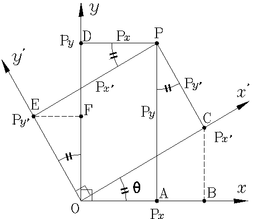
\[ \begin{bmatrix} P_x \\ P_y \end{bmatrix} = \begin{bmatrix} \cos\theta & -\sin\theta \\ \sin\theta & \cos\theta \end{bmatrix} \begin{bmatrix} P_{x'} \\ P_{y'} \end{bmatrix} \tag{a} \]

Therefore,

\[ \begin{bmatrix} P_{x'} \\ P_{y'} \end{bmatrix} = \begin{bmatrix} \cos\theta & \sin\theta \\ -\sin\theta & \cos\theta \end{bmatrix} \begin{bmatrix} P_x \\ P_y \end{bmatrix} \]

or

\[ \mathbf{P'} = \mathbf{TP} \tag{b} \]

In the transformation matrix \(\mathbf{T}\) of Equation (b), the inner product of the two row vectors is zero, and the magnitude of each row vector is 1. The transformation matrix is therefore an orthonormal matrix. Since the inverse of an orthonormal matrix is equal to its transpose,

\[ \mathbf{T}^{-1} = \mathbf{T}^{\text{T}} \tag{c} \]

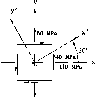
Stress, which is described as the force acting per unit area, is a mechanical quantity defined not only by the magnitude and direction of the force but also by the direction and magnitude of the area. A single stress state having the same physical meaning is expressed by different component values depending on the coordinate system. For example, if the stress components in the \(x-y\) coordinate system of Figure A.1 are \(\sigma_{xx} = 110.0\,\text{MPa}\), \(\sigma_{yy} = 50.0\,\text{MPa}\), \(\sigma_{xy} = 40.0\,\text{MPa}\), then the components with respect to the \(x'-y'\) coordinate system are given by the following relation,

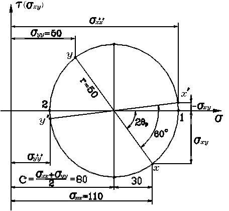
\[ \begin{bmatrix} \sigma_{x'x'} & \sigma_{x'y'} \\ \sigma_{y'x'} & \sigma_{y'y'} \end{bmatrix} = \begin{bmatrix} \cos\theta & \sin\theta \\ -\sin\theta & \cos\theta \end{bmatrix} \begin{bmatrix} \sigma_{xx} & \sigma_{xy} \\ \sigma_{yx} & \sigma_{yy} \end{bmatrix} \begin{bmatrix} \cos\theta & -\sin\theta \\ \sin\theta & \cos\theta \end{bmatrix} \tag{A.4} \]

yielding \(\sigma_{x'x'} = 129.6\,\text{MPa}\), \(\sigma_{y'y'} = 30.4\,\text{MPa}\), \(\sigma_{x'y'} = -6.0\,\text{MPa}\). These values can also be obtained using Mohr's circle, as in Example A.3. Mohr's circle is a geometric representation of the above transformation relation.

Example A.3

When the stress components with respect to the \(x-y\) coordinate system are \(\sigma_{xx} = 110.0\,\text{MPa}\), \(\sigma_{yy} = 50.0\,\text{MPa}\), \(\sigma_{xy} = 40.0\,\text{MPa}\), use Mohr's circle to find the principal stresses and the stress components with respect to the \(x'-y'\) coordinate system of Figure A.1.

Solution

The center \((c, 0)\) and radius \(r\) of Mohr's circle are

\[ c = (\sigma_{xx} + \sigma_{yy})/2 = 80.0 \tag{a} \]

\[ r = \left( (\sigma_{xx} - \sigma_{yy})^2 / 4 + \sigma_{xy}^2 \right)^{0.5} = 50.0 \tag{b} \]

so that

\[ \begin{aligned} \sigma_{x'x'} &= c + r \cos(60^\circ - 53.13^\circ) = 129.6\,\text{MPa} \\ \sigma_{y'y'} &= c - r \cos(60^\circ - 53.13^\circ) = 30.4\,\text{MPa} \\ \\ \sigma_{x'y'} &= -r \sin(60^\circ - 53.13^\circ) = -6.0\,\text{MPa} \end{aligned} \tag{c} \]

The magnitudes and directions of the principal stresses are as follows.

\[ \begin{aligned} \sigma_1 &= c + r = 130.0 \\ \sigma_2 &= c - r = 30.0 \end{aligned} \tag{d} \]

\[ \theta_p = \frac{1}{2} \tan^{-1} (2\sigma_{xy} / (\sigma_{xx} - \sigma_{yy})) = 26.6^\circ \tag{e} \]

Therefore, the maximum principal stress axis lies in the direction obtained by rotating the \(x\)-axis counterclockwise by \(26.6^\circ\).

In the foregoing, we studied that if a mechanical quantity at a material point is expressed on the basis of two different coordinate systems, the two representations of the quantity must satisfy the transformation relation defined by the difference between the coordinate systems. This transformation relation will be explained in more detail later. From the standpoint of the aforementioned transformation relation, all mechanical quantities receive the same mathematical treatment and are collectively referred to as tensor quantities. Only the form of the transformation differs. As seen in Equation (A.1), a scalar quantity does not use a transformation matrix, so it is called a tensor of order zero; a vector quantity has a first-order transformation relation involving a single transformation matrix, as seen in Equation (A.2), so it belongs to the tensors of order one (first-order tensors). Stress and the like have a second-order transformation relation using two transformation matrices, as seen in Equation (A.4), so they are tensors of order two. The transformation relations for tensor quantities are detailed separately. It should be emphasized here that, in continuum mechanics including solid mechanics, mechanical quantities are expressed as functions of coordinates and are, from the standpoint of coordinate transformation, mathematically identical tensor quantities.

Example A.5

Understand the following relations.

Solution

a) \(\delta_{12} = 0\)

b) \(\delta_{22} = 1\)

c) \(\displaystyle\sum_{i=1}^{3} \delta_{ii} = 3\)

d) \(\displaystyle\sum_{j=1}^{3} \delta_{1j} u_j = u_1\)

e) \(\displaystyle\sum_{j=1}^{3} \delta_{ij} u_j = u_i\)

Partial-derivative terms with respect to coordinates appear frequently in the formulas of mechanics problems. In index notation, a comma (,) and the indices following the comma are used to express partial differentiation concisely. The comma separates the function being differentiated (a component of a mechanical quantity) from the differentiation coordinate. That is, the indices before the comma are the numbers denoting the components of the tensor quantity, and the indices after the comma are the numbers designating the differentiation coordinate or variable.

Example A.6

Master the partial-differentiation convention through the following examples.

Solution

\[ \text{a) } \phi_{,i} = \frac{\partial\phi}{\partial x_i} , \quad \phi_{,2} = \frac{\partial\phi}{\partial x_2} \]

\[ \text{b) } v_{i,j} = \frac{\partial v_i}{\partial x_j} \]

\[ \text{c) } \sigma_{ij,j} = \frac{\partial\sigma_{ij}}{\partial x_j} \]

\[ \text{d) } \varepsilon_{ij,kl} = \frac{\partial^2\varepsilon_{ij}}{\partial x_k \partial x_l} \]

\[ \text{e) } x_{i,j} = \frac{\partial x_i}{\partial x_j} = \delta_{ij} \]

\[ \text{f) } \sigma_{ij} w_{i,j} = (\sigma_{ij} w_i)_{,j} - \sigma_{ij,j} w_i = \frac{\partial(\sigma_{ij} w_i)}{\partial x_j} - \frac{\partial\sigma_{ij}}{\partial x_j} w_i \]

In most formulas of mechanics problems, a summation symbol (\(\sum\)) precedes the expression, and in most cases the index used for summation appears twice within a single term. The equilibrium equation

\[ \sum_{j=1}^{3} \sigma_{ij,j} + f_i = 0 \tag{A.7} \]

is one example. Under the summation convention, if two identical indices appear in a single term, the summation symbol may be omitted. In this case such an index is called a dummy index, and when a single index appears in a term that is not preceded by a summation symbol it is called a free index. A dummy index can always be replaced by another index as long as its meaning is not lost, whereas when a free index is changed, the same index in all terms must be changed simultaneously. Moreover, the same free index must necessarily be present in every term of the expression.

In this book, when the same index appears three times in a single term, as in \(\displaystyle\int_{S_{\sigma_i}} \bar{t}_i u_i \, dS\), but one of those indices is used to express the integration domain, the expression is regarded as following the summation convention.

Example A.7

Point out what is wrong in the following expressions.

a) \(\sigma_{ij,j} + f_j = 0\)

b) \(\sigma_{ij} = 2\mu\varepsilon_{ij} + \lambda\varepsilon_{ii}\delta_{ij} - (3\lambda + 2\mu)\alpha \, \Delta T \delta_{ij}\)

Solution

a) In the first term, \(i\) is a free index and \(j\) is a dummy index. Since the same free index must be present in every term, the free index \(i\) must necessarily be present in the second term. Therefore, the subscript \(j\) in \(f_j\) must be changed to \(i\). That is, \(\sigma_{ij,j} + f_i = 0\) is the correct expression.

b) On the left-hand side, \(i\) and \(j\) are free variables. In the first and third terms of the right-hand side, the same free variables as on the left-hand side are present, so there is no problem with the expression. On the other hand, in the second term, \(i\) is repeated three times, so \(i\) is neither a free index nor a dummy index. Therefore, it suffices to change \(\varepsilon_{ii}\) to \(\varepsilon_{kk}\) (see Section 5.3).

Example A.8

The following are examples of the summation convention frequently used in advanced mechanics. Through understanding these examples, become familiar with the summation convention and index notation.

Solution

\[ \text{a) } \sigma_{kk} = \sum_{k=1}^{3} \sigma_{kk} = \sigma_{jj} = \sigma_{ii} = \sigma_{11} + \sigma_{22} + \sigma_{33} \, (= \sigma_{xx} + \sigma_{yy} + \sigma_{zz}) \tag{a} \]

\[ \text{b) } \sigma_{ij,j} = \sum_{j=1}^{3} \sigma_{ij,j} = \sigma_{ik,k} = \frac{\partial\sigma_{i1}}{\partial x_1} + \frac{\partial\sigma_{i2}}{\partial x_2} + \frac{\partial\sigma_{i3}}{\partial x_3} \tag{b} \]

\[ \text{c) } u_{i,i} = \sum_{i=1}^{3} u_{i,i} = u_{j,j} = \frac{\partial u_1}{\partial x_1} + \frac{\partial u_2}{\partial x_2} + \frac{\partial u_3}{\partial x_3} = \frac{\partial u_x}{\partial x} + \frac{\partial u_y}{\partial y} + \frac{\partial u_z}{\partial z} \tag{c} \]

\[ \text{d) } \varepsilon_{ii} = \varepsilon_{11} + \varepsilon_{22} + \varepsilon_{33} = u_{i,i} \tag{d} \]

\[ \text{e) } \delta_{ii} = \sum_{i=1}^{3} \delta_{ii} = \delta_{kk} = 3 \tag{e} \]

\[ \text{f) } \delta_{ij} u_j = \sum_{j=1}^{3} \delta_{ij} u_j = \delta_{i1} u_1 + \delta_{i2} u_2 + \delta_{i3} u_3 = u_i \tag{f} \]

\[ \text{g) } \sigma_{ij} n_i n_j = \sum_{i=1}^{3} \sum_{j=1}^{3} \sigma_{ij} n_i n_j \tag{g} \]

\[ \text{h) } \sigma_{ij} n_j = \sum_{j=1}^{3} \sigma_{ij} n_j = \sigma_{ik} n_k \tag{h} \]

\[ \text{i) } \varepsilon_{ij} \delta_{ij} = \varepsilon_{ii} \text{ or } \varepsilon_{jj} \tag{i} \]

\[ \text{j) } \mathbf{t}^{(\mathbf{n})} = \sigma_{ij} \mathbf{e}_j = \sigma_{i1} \mathbf{e}_1 + \sigma_{i2} \mathbf{e}_2 + \sigma_{i3} \mathbf{e}_3 \tag{j} \]

\[ \text{k) } x'_i = T_{ij} x_j = T_{i1} x_1 + T_{i2} x_2 + T_{i3} x_3 \tag{k} \]

\[ \text{l) } \int_{S_{\sigma_i}} \bar{t}_i u_i \, dS = \int_{S_{\sigma_1}} \bar{t}_1 u_1 \, dS + \int_{S_{\sigma_2}} \bar{t}_2 u_2 \, dS + \int_{S_{\sigma_3}} \bar{t}_3 u_3 \, dS \tag{l} \]