12 Modeling of Materials
12.1 Elastic Deformation and Plastic Deformation
In the tensile testing of metals, there is a clearly identifiable region in which stress and strain can be regarded as varying linearly. The limit of this region is called the proportional limit. Beyond it, the behavior becomes nonlinear, and once the yield point is reached, permanent deformation occurs. This permanent deformation is called plastic deformation. In the elastic deformation region, the deformation is regarded as sufficiently small, and the true stress and true strain are assumed to be identical to the nominal stress and nominal strain, respectively. In most structural mechanics, there is no interest in stresses above the proportional limit, so nonlinear elasticity is neglected. Even in plasticity mechanics, where its influence is relatively large, nonlinear elastic behavior is neglected.
In bulk metal forming, it is common for the local maximum strain to reach 2.0 or more. In contrast, the strain at the yield point does not exceed 0.005. When the elastic modulus of steel is taken as 200 GPa, a strain of 0.005 at the yield point corresponds to a yield strength of 1000 MPa. In cold forging, which generally attaches importance to the influence of elastic deformation, the flow stress including the initial yield stress is lowered through heat treatment such as annealing, so 1000 MPa is not a small value. Therefore, the rigid-plastic assumption, which neglects the influence of elastic deformation during metal forming, is generally adopted. The rigid-plastic assumption can be effective, owing to the advantages of rigid-plasticity, for predicting the shape of the material and predicting the load. However, it has limitations in solving problems where residual stress and springback are important.
Characterizing the behavior of materials at high strains is not easy. This is because, in widely known material testing methods, the maximum reliable strain is smaller than expected. In a tensile test, the maximum strain at the fracture surface may reach 1.5 or more, but the true strain up to the necking point, where hand calculation of the true stress is possible, mostly does not reach 0.15. In a compression test, once the true strain reaches 0.5 or more, homogeneity deteriorates due to barreling of the specimen and the increasing influence of friction, so the true strain–true stress relationship cannot be obtained by hand calculation. Theoretically, a torsion test can subject the material to relatively high strains, but the torsion test is used only in a limited way for the purpose of obtaining flow stress.
Therefore, the flow stress at high strain can only be estimated using flow stress information at low strain. In a tensile test, the material undergoes large strain near the necking point just before fracture. Taking advantage of this, various researchers have proposed methods for obtaining flow stress at high strain based on the tensile test.
12.2 Deformation Characteristics of Steel with Temperature
The elastic and plastic deformation characteristics of metals change sensitively with temperature. Strictly speaking, the elastic modulus and Poisson's ratio are also functions of temperature. In particular, ductility, which is regarded as important among the macroscopic properties of steel, is also strongly related to temperature. Figure 12.1 shows the ductility of steel as a function of temperature [12.1]. Overall, the elongation increases as the temperature rises, but it can be seen that the elongation decreases locally in the blue-brittleness region around 300°C. To prevent fracture of the material during cold forging, this region must be avoided. As blue brittleness is passed, the elongation continues to increase, and when the allotropic transformation region is reached, the elongation decreases sharply. Plastic forming carried out in these two brittleness regions is called warm metalworking. Beyond the allotropic transformation, the elongation increases, and when the hot-brittleness region is reached, the elongation decreases sharply. Hot plastic forming carried out while avoiding the allotropic transformation region and the hot-brittleness region is called hot metalworking.
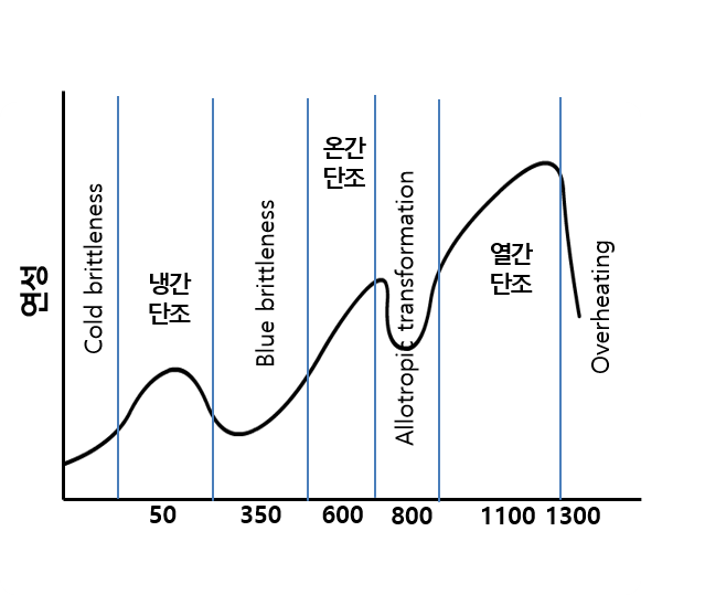
Figure 12.1 Correlation between temperature and elongation of steel [12.1]
In general, the flow stress or deformation resistance of a metal decreases as the temperature rises. Figure 12.2 shows the change in the flow stress of S35C and three stainless steels with changing temperature [5.1].
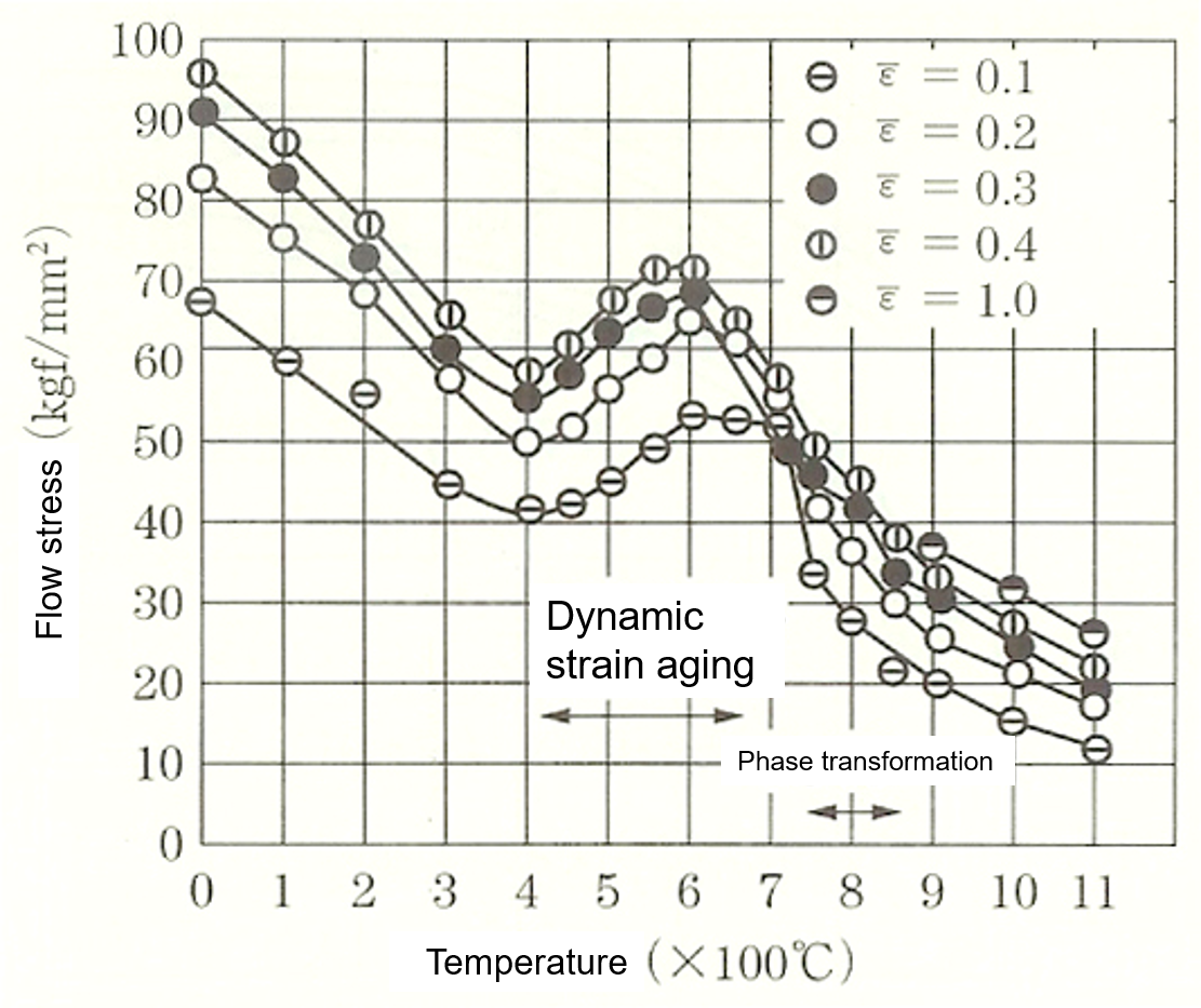
⒜ S35C, effective strain rate = 450 /s 12.1
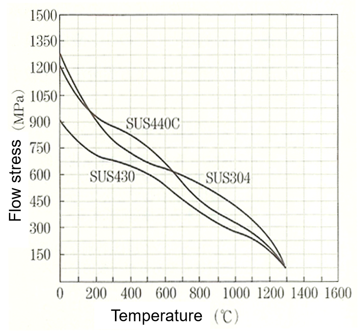
⒝ strain = 1.0
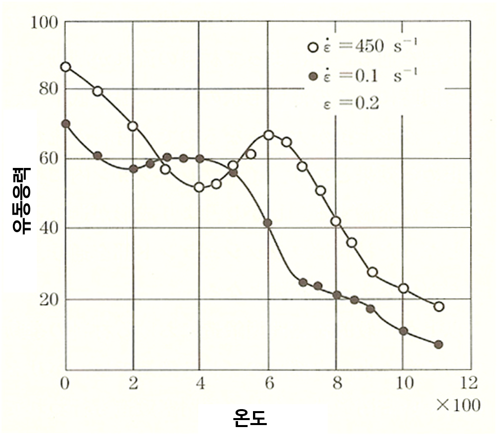
⒞ S35C, strain = 0.2, strain rate 0.1/s and 450/s
Figure 12.2 Effect of temperature on flow stress [5.1]
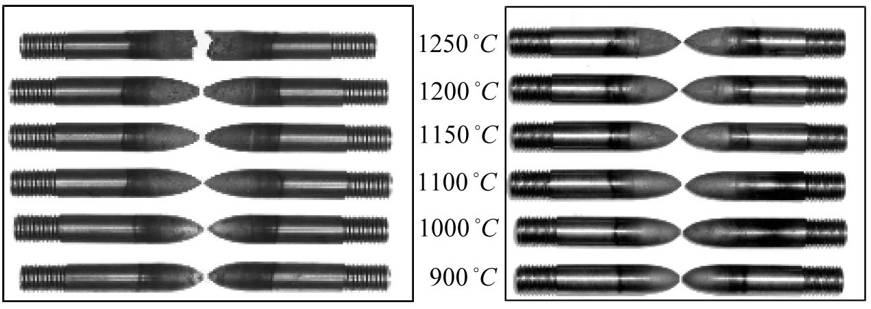
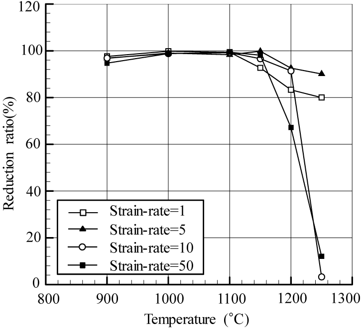
It can be seen that the flow stress decreases greatly as the temperature rises. As the temperature rises from 0°C to 1100°C, the flow stress decreases to one-fourth to one-sixth. Utilizing this characteristic of flow stress, bulky formed products are formed by hot metalworking. This is to reduce the press load and prevent damage to the die. In Figure 12.2⒜, there is a region around 400°C where the flow stress locally rises as the temperature increases. This implies that the flow stress is in a sensitive functional relationship not only with temperature but also with strain and strain rate. Obtaining this functional relationship requires precision testing equipment together with specialized knowledge. Therefore, the degree of understanding of this functional relationship is directly linked to the engineer's competence. The hot-brittleness region differs greatly depending on the composition of the material. For example, when the temperature of STB2 reaches 1200°C, the elongation drops sharply. The high-temperature elongation can be obtained relatively easily by a high-temperature tensile test. Since the high-temperature elongation is sensitive to temperature, experimental investigation of it must precede hot metalworking. In the high-temperature state, recrystallization occurs continuously in the material, so the strain-hardening capacity drops greatly. Therefore, necking occurs early during a tensile test. Hence, obtaining the flow stress from information prior to the onset of necking is meaningless. And even after the onset of necking, because of the strong dependence on strain and strain rate, obtaining the flow stress from tensile test information is not easy. However, the high-temperature tensile test of a material is useful for the purpose of evaluating the forgeability of the material at high temperature. Here, the importance of the high-temperature tensile test is emphasized through an example. That is, a case study [12.2] on the evaluation of the formability and hot brittleness of bearing steel through a tensile test is introduced. The bearing materials used in the test are STB2 and SCM420H. Tensile tests were conducted under various conditions of temperature (900, 1000, 1100, 1150, 1200, 1250 °C) and strain rate (1, 5, 10, 50 /s). The diameter of the specimen used in the tensile test is 10 mm and the length is 110 mm. As shown in Figure 12.3, even though both are bearing steels, their deformation characteristics at high temperature differ greatly. From Figure 12.3⒜, it can be understood why the forging temperature of STB2 must be controlled to below 1200°C, including the temperature rise due to plastic heat. To quantitatively evaluate the tensile test results, the change in the reduction of area () with temperature was examined. The reduction of area is defined as follows.
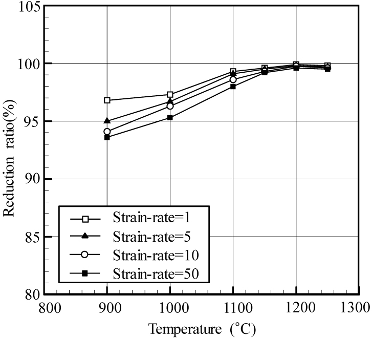
Here, \(A_o\) and \(A_f\) are the initial cross-sectional area and the cross-sectional area at fracture of the specimen, respectively. The reduction of area is proportional to the ductility. For the STB2 bearing steel in Figure 12.4⒜, the reduction of area increases as the temperature rises, but after about 1150°C the reduction of area decreases, and in particular, when the strain rate is high, the reduction of area decreases sharply. In contrast, for the SCr420H bearing steel in Figure 12.4⒝, the reduction of area continuously increases as the temperature rises, and the reduction of area was large even at 1200°C and 1250°C.
(a) STB2
⒝SCr420H
Figure 12.4 Variation of the reduction of area with temperature
12.3 Flow Stress
12.3.1 Introduction
In metal forming, the core of the material properties is the flow stress. The flow stress has a large effect on the analysis results, and although it shows relatively minor differences depending on the type of material, the influence of temperature is decisive. As shown in Figure 12.2, the flow stress of a material changes greatly with temperature. In steel, transformation occurs, so an abrupt change in flow stress occurs before and after the transformation point, but overall it shows a proportional relationship with temperature. These figures clearly show that hot forging and cold forging will differ greatly in terms of forming load. Of course, a large forming load requires correspondingly large energy and power. In practice, cold forging is applied only to small products because of limitations in forming load, energy, and power. Recently, cold forging machines of around 2500 tons have become available, but there is inevitably a constraint on the size of the product. Therefore, based on Japan's forging production in 2002, as shown in Figure 12.5, the proportion accounted for by hot forging is overwhelmingly large (the fastener manufacturing industry was excluded from these statistics). The properties of a material at room temperature are expressed by strain-hardening capacity or strain-hardening characteristics, and the properties of a material at high temperature are represented by viscosity. For example, if 'plastic' is attached to a material model name, it means that there is strain-hardening capacity (strain dependence), and if there is no strain-hardening capacity, the term 'perfectly plastic' is used. If 'visco' is attached to a material model name, it means that there is a viscous property (strain-rate dependence). That is, it means that the deformation of the material is dependent on the strain rate. And if 'thermo' is attached to a material model name, it means that it is influenced by temperature. Therefore, the term 'thermoviscoplastic' is used when the material is dependent on temperature, strain rate, strain, etc., and 'rigid-thermoviscoplastic finite element method' and 'elastothermoviscoplastic finite element method' are translated as the rigid-thermoviscoplastic finite element method and the elastothermoviscoplastic finite element method, respectively. The former refers to a finite element method that uses a material model neglecting elastic deformation while considering the influence of temperature, strain rate, and strain, and the latter is the case where the influence of elastic deformation is considered. These two terms also apply when the strain dependence of the material, i.e., strain hardening, is neglected.
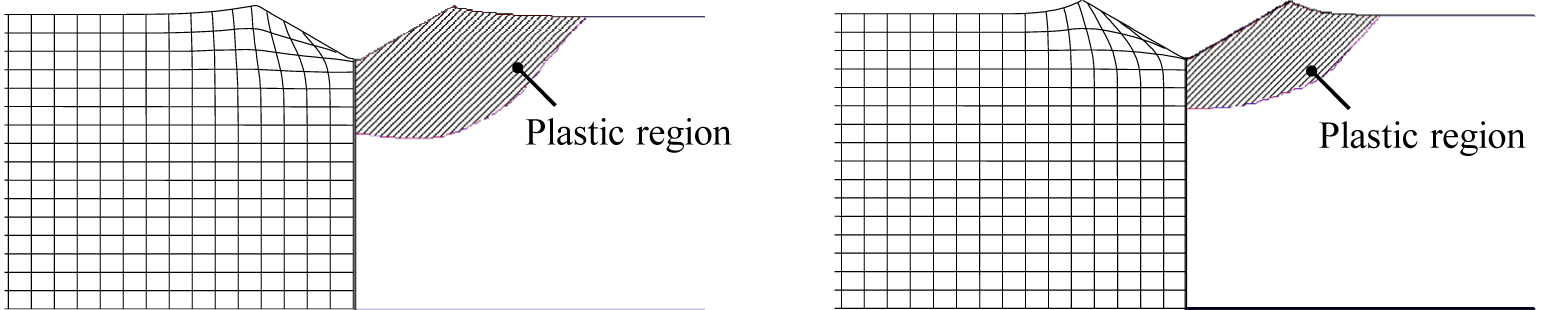
Figure 12.5 Production of forged products by forging method [5.1]
Obtaining the flow stress is done by material testing including tensile tests, compression tests, and torsion tests. For the flow stress of a material at room temperature, all experimental methods are valid, but at high temperature the tensile test is not valid for the purpose of obtaining flow stress. However, when one wishes to characterize the high-temperature fracture behavior and hot brittleness of a material, the tensile test is valid.
In practice, for the purpose of obtaining the flow stress, the compression test is generally relied upon even at room temperature. The reasons are that the experiment is relatively simple and that experimental values for medium-magnitude strains can be obtained. Of course, at high temperature, necking occurs early, so it is not easy to obtain flow-stress-related information by tensile testing.
Expressing the flow stress as a formula (flow stress modeling) is important for the purpose of process analysis and for characterizing the plastic deformation behavior of the material. Many researchers have proposed functional relationships between the flow stress and the state variables, i.e., material flow stress model formulas. Flow stress models are based on metallurgical and phenomenological backgrounds, and most room-temperature flow stress models and many high-temperature flow stress models are based on phenomenological backgrounds. A flow stress model consists of known functions and unknown constants, and these unknown constants can be regarded as part of the material properties. They play a role similar to the elastic modulus and Poisson's ratio required in the elasticity of isotropic materials.
modulus and Poisson's ratio, and play a similar role.
Many flow stress models have an application temperature range suitable for the model, and there also exist flow analysis models with a wide range of applicability covering both room temperature and high temperature, such as the Johnson–Cook model.
The higher the degrees of freedom of a flow stress model, i.e., the more variables that must be determined, the more advantageous it is for expressing a flow stress closer to reality, but the problem is that obtaining the complex functional relationship, i.e., the many coefficients that determine the material properties, requires great expense.
Therefore, it is desirable to express the flow stress with accuracy suitable for the purpose, centering on the main variables. In general, strain, strain rate, temperature, etc., have a large effect on the flow stress. In some cases, there is a tendency to neglect the influence of temperature even in hot or warm forming. This is because, even so, the information required in process development, in particular the approximate results for the flow lines and forming load, can be obtained.
To explain concretely, this is because the incompressibility condition imposed by the theory strongly induces the material to essentially flow into the empty space formed by the die and the material. Even if this flow produces a slight local error, the flow of the material satisfying the incompressibility condition does not cause a large problem in terms of the macroscopic result. Therefore, appropriate constraints or assumptions regarding the flow stress are needed depending on the purpose of the process analysis. This is because the analysis results are ultimately given meaning through judgment based on the engineer's experience, so obtaining a controllable and stable theoretical solution that retains only the main variables is more important.
12.3.2 Room-Temperature Flow Stress
12.3.2.1 Strain-Hardening Capacity and Plastic Flow
The most important factor in the plastic flow characteristics of metals at room temperature is strain hardening. Plastic deformation is accompanied by the generation of dislocations, and strain hardening is a metallurgical and mechanical phenomenon in which the dislocation density increased by plastic deformation hinders the generation or growth of new dislocations, thereby increasing the material's resistance to deformation. increases—a metallurgical and mechanical phenomenon. First, to visualize the influence of the strain-hardening exponent, a case study is introduced in which SCM435, which has a large strain-hardening capacity, and ESW105, whose strain-hardening capacity is negligibly small, are applied to various processes. duced. In cold metal forming, the main factor determining flow stress and plastic flow is strain. The value representing the strain dependence of flow stress is the strain-hardening exponent. Figure 12.6 emphasizes the difference between a typical strain-hardening material and a material with almost no hardening capacity (see Figure 12.9⒝). That is, the plastic flow patterns occurring during an indentation test with a cone of 120° apex angle were compared; a material with large strain hardening has the property that the deformation resistance increased due to prior plastic deformation tends to propagate the deformation relatively widely. In contrast, a low-strain-hardening material shows a tendency for plastic deformation to concentrate in the main deformation region. This can produce relatively large differences in plastic flow in regions where local underfill occurs or where deformation is locally concentrated. In conclusion, the strain-hardening exponent in the flow stress has the largest effect on the analysis results, and is the factor with the greatest influence on identifying the causes of local defects, buckling, and internal and external cracks.
Figure 12.6 Metal flow lines in the conical indentation test
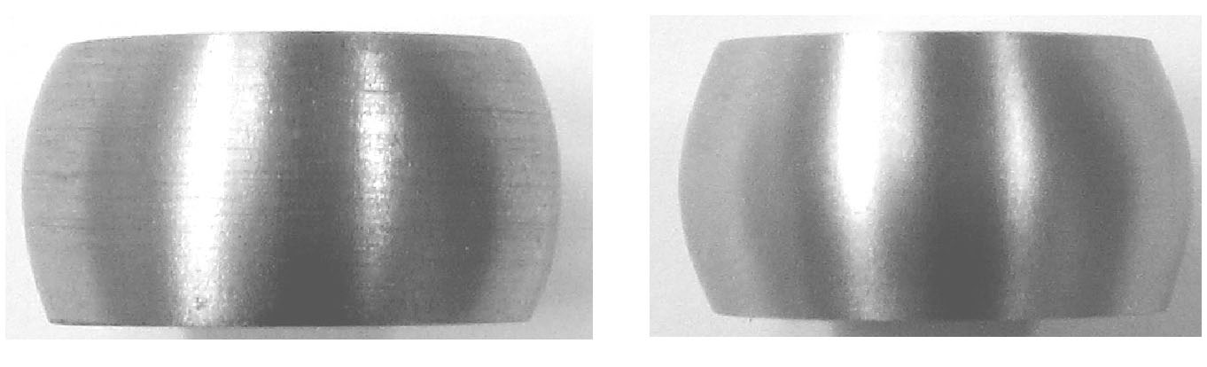
Most forging processes involve axial compression of a cylinder, i.e., upsetting. This is generally because the diameter of the material is standardized, whereas the diameter of the product varies widely. That is, the work of matching the material diameter through a cylinder compression process usually precedes. Of course, upsetting is also widely performed for the purpose of improving the surface and shape quality of the fracture surface. Here, the barreling phenomenon occurring during cylinder upsetting was investigated through experiment and simulation. The diameter and height of the cylindrical specimen were set to 16 mm and 24 mm, respectively, and no coating treatment was applied. The friction coefficient was taken as 0.15. This value is between 0.1 and 0.2, the friction coefficient when unlubricated steel contacts steel at room temperature [12.3]. Compression was performed so that the reduction ratio (height reduction ratio) was 50%. The analysis results and experimental results are shown in Figures 12.7⒜ and 12.7⒝, respectively. From the analysis results in Figure 12.7⒜ obtained under the same conditions, it can be seen that although the diameters of the parts in contact with the upper and lower dies are similar, the specimen of the low-strain-hardening material has a greater amount of protrusion at the middle part during barreling than the specimen of the high-strain-hardening material. This is a result implying that the specimen of the high-strain-hardening material forms a smoother curved surface. This phenomenon also appears in the experimental results of Figure 12.7⒝. Such plastic deformation behavior can act as a favorable condition or an unfavorable condition depending on the shape of the product. An easily conceivable point is that when forging a low-strain-hardening material, the amount of upsetting must be relatively small. This will act unfavorably in the problem of filling corners. Of course, in processes where the flash problem that occurs when corners fill first is serious, a low-strain-hardening material may be more advantageous.
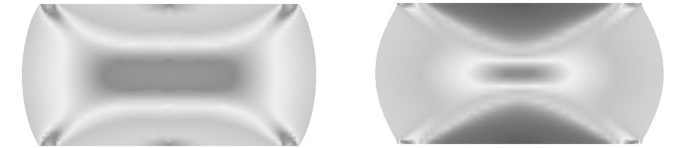
⒜ Analysis results
 s
s
(b) Experimental results
Figure 12.7 Experimental results of the axial compression test
And to analyze the influence of strain hardening in an actual process, the ball-stud forging processes of SCM435 and ESW105 were simulated and the results were compared. The Coulomb friction law was used, and the friction coefficient was assumed to be \(\mu = 0.05\). The target process consists of four stages. The process diagram is shown in Figure 12.8⒜, and the main results are compared in Figures 12.8⒝ and 12.8⒞. Figure 12.8⒝ shows the contact stress acting on the die in the third and fourth stages. Figure 12.8⒞ shows the history of the forming load. As shown in the figures, it can be confirmed that the contact stress and forming load for the two materials differ greatly. Process design is inseparably related to material flow. If die deformation is neglected, the plastic flow characteristics of the material are absolutely influenced by the strain-hardening capacity. Even if the types of materials differ, if the strain-hardening exponents are similar, the deformed shapes are inevitably similar. When the strain-hardening exponent is inherently small, as in non-heat-treated steel or pre-quenched-and-tempered steel, or when hardening has already occurred in a process such as drawing and the strain-hardening capacity in the subsequent plastic deformation has been artificially lowered, the material may differ in terms of plastic flow from a material of similar composition.
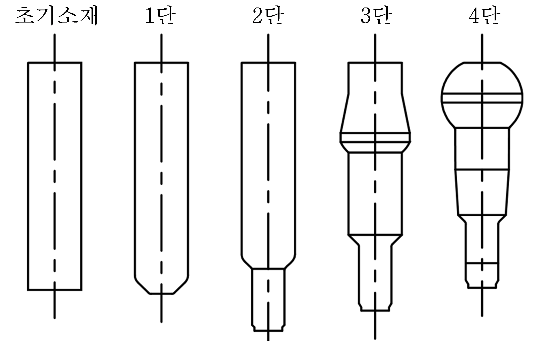
⒜ Ball-stud process design diagram
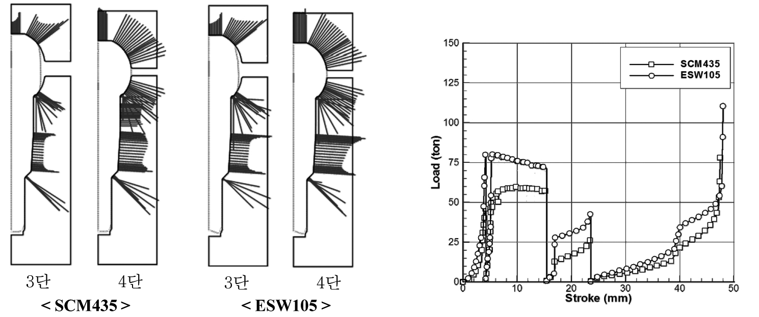
⒝ Comparison of contact stress acting on the die-material interface ⒞ Comparison of forming load-stroke curves
Figure 12.8 Ball-stud cold forging
The foregoing is not intended to compare the materials. It is to emphasize that the macroscopic characteristics of the two materials differ. However, it is emphasized that process design for two materials with different characteristics must be done from completely different angles. When a process designer familiar with the SCM435 material designs for a material such as SEW105, they must rely more on scientific analysis technology than on prior experience. Otherwise, it will be difficult to meet the demands of the era for new materials that are difficult to form.
12.3.2.2 Room-Temperature Flow Stress Model
As explained in Section 12.3.2.1, the plastic deformation of metal materials at room temperature is closely related to strain. This functional relationship must be expressed in an applicable manner. A representative one used is the closed-form function. In cold working processes, the flow stress is generally regarded as a function of the effective strain only, and the relevant coefficients can be easily obtained through tensile tests, compression tests, etc. The following formulas are widely used as mathematical models for modeling the flow stress of cold materials.
In cold working processes, the flow stress is generally regarded as a function of the effective strain only, and the relevant coefficients can be easily obtained through tensile tests, compression tests, etc. The following formulas are widely used as mathematical models for modeling the flow stress of cold materials.
Here, \(Y_o\) is the initial yield stress, and \(K\) and \(n\) are called the strength coefficient and the strain-hardening exponent, respectively. Among these, Eq. (12.3) is the most widely used. Eq. (12.2) is called Swift's flow stress equation, Eq. (12.3) is called Hollomon's flow stress equation, and Eq. (12.4) is called Ludwik's flow stress equation. According to theory, the strain-hardening exponent \(n\) coincides with the true strain \(\varepsilon_N\) at the point where necking occurs during a tensile test. That is,
This is called the Considère condition [12.4].
However, the value obtained by Eq. (12.6) and the value obtained by curve fitting differ somewhat in practice. Nevertheless, the value determined by Eq. (12.6) predicts the onset of necking relatively accurately in the simulation of a tensile test [12.5]. Therefore, in problems where the onset of necking and the deformation shape and behavior of the specimen due to necking are important, the strain-hardening exponent of Eq. (12.6) is used, and when overall flow stress information is desired for application to metal forming processes, it is desirable to use material constants obtained by considering the overall behavior of strain and flow stress. To solve this problem with a single formula, the following improved model of the Hollomon model has been developed and used [12.6].
The feature of this model is that, by using an appropriate functional relationship of \(K\) and \(n\), it accurately predicts the necking point in the tensile test while also solving the problem of underestimating the flow stress after necking. The details of this mathematical model are described in Section 12.5.
In cold working, the velocity dependence of the material is neglected in most cases. However, there may be cases in actual cold forming where the velocity dependence cannot be neglected. In particular, the flow stress of aluminum changes sensitively with temperature, and temperature is relatively strongly influenced by velocity. Therefore, the selection of the main variables suited to the situation is important. Figure 12.9 shows experimental results of the velocity dependence of commercial steel and an example of a flow stress model and its formulation. The flow stress model formula used in this figure, Eq. (12.8), regards the strength coefficient and strain-hardening exponent in the traditional Hollomon model as functions of strain rate and temperature. In fact, only the strain-rate dependence was considered in Figure 12.9. If the temperature dependence is considered, the temperature dependence of the flow stress at room temperature can be reflected, as shown in Figure 12.2.
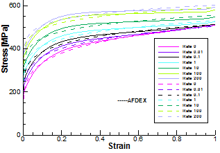
Figure 12.9 Experimental values (solid lines) and formulation results (dashed lines) of the velocity dependence of commercial steel
In addition to the room-temperature flow stress models described above, many phenomenological and practical formulas or techniques are used. A representative one is a method that uses the Hollomon formula but calculates the strength coefficient and strain-hardening exponent from the two pieces of information, the yield strength and tensile strength. This flow stress model requires the yield strength and tensile strength as inputs, but is in fact the Hollomon flow stress model. And the flow stress can also be defined by a point cloud of (strain, flow stress) obtained based on experimental results.
12.3.3 High-Temperature Flow Stress
12.3.3.1 Main Factors Affecting the High-Temperature Flow Stress
What distinguishes commercial metal materials in the high-temperature state from those at room temperature is recrystallization. Even at room temperature, the flow stress of a material is temperature-dependent and has the property of resisting velocity. The problem is the degree of this. However, recrystallization is a completely different matter. Of course, there are also metals that undergo recrystallization even at room temperature, but that is exceptional.
At high temperature under low strain, the material undergoes the same strain-hardening history as at room temperature. However, once the peak strain is reached, it undergoes deformation softening due to recrystallization, and reaches a state where strain hardening and softening are balanced, i.e., a steady state.
Of course, at high temperature metal materials are much more sensitive to temperature than at room temperature. As shown in Figure 12.2(c), when steel is heated from \(0^\circ\text{C}\) to \(100^\circ\text{C}\) at low speed, the flow stress decreases by about 15%, whereas when heated from \(1000^\circ\text{C}\) to \(1100^\circ\text{C}\), the flow stress decreases by about 40%. And when the material is overheated, the hot-brittleness region, where elongation drops sharply, awaits. For this reason, temperature is regarded as important in hot metalworking.
Similarly, the influence of strain rate also increases toward higher temperatures. As shown in Figure 12.2(c), it can be seen that the difference in flow stress due to velocity increases toward higher temperatures. The difference between the low strain rate (\(0.1/\text{s}\)) and the high strain rate (\(450.0/\text{s}\)) at \(0^\circ\text{C}\) is about 15%, but at \(1000^\circ\text{C}\) that difference is about 50%, and it can be confirmed that the ratio increases as the temperature increases.
Although the flow stress is greatly influenced by temperature, isothermal analysis using an average temperature is widely used. The analysis of metal forming processes is divided into non-isothermal analysis and isothermal analysis. The analysis of hot forging processes also belongs to isothermal analysis when it is analyzed neglecting the influence of temperature. In isothermal forging and superplastic forming, the forming temperature is kept constant. Even in such processes, when one wishes to predict partial temperature changes, non-isothermal analysis must be performed.
On the surface of the material in contact with the die during hot metalworking, the temperature drops sharply, while deep inside the temperature rises due to plastic heat. If no heat conduction occurred, in a region where the flow stress of steel is 125.0 MPa and the effective strain reaches 2.5, the local temperature rise due to plastic heat would reach \(\Delta T = 2.5 \times 125.0 / (0.0052 \times 1000.0) = 60^\circ\text{C}\) according to the following equation. Even taking heat conduction into account, a considerable amount of temperature rise is unavoidable [12.2].
Here, \(\bar{\sigma}\) is the average flow stress, \(\bar{\varepsilon}\) is the effective strain, and \(\rho c\) is the heat capacity.
Because the temperature rise at the surface causes an increase in the flow stress of the material, it will act to impede material flow at the surface. However, this is linked with the friction law, so it is difficult to distinguish its influence. If a hot forging process is analyzed by isothermal analysis neglecting the influence of temperature, making the friction coefficient slightly larger than the actual value can yield more realistic results in terms of the flow lines.
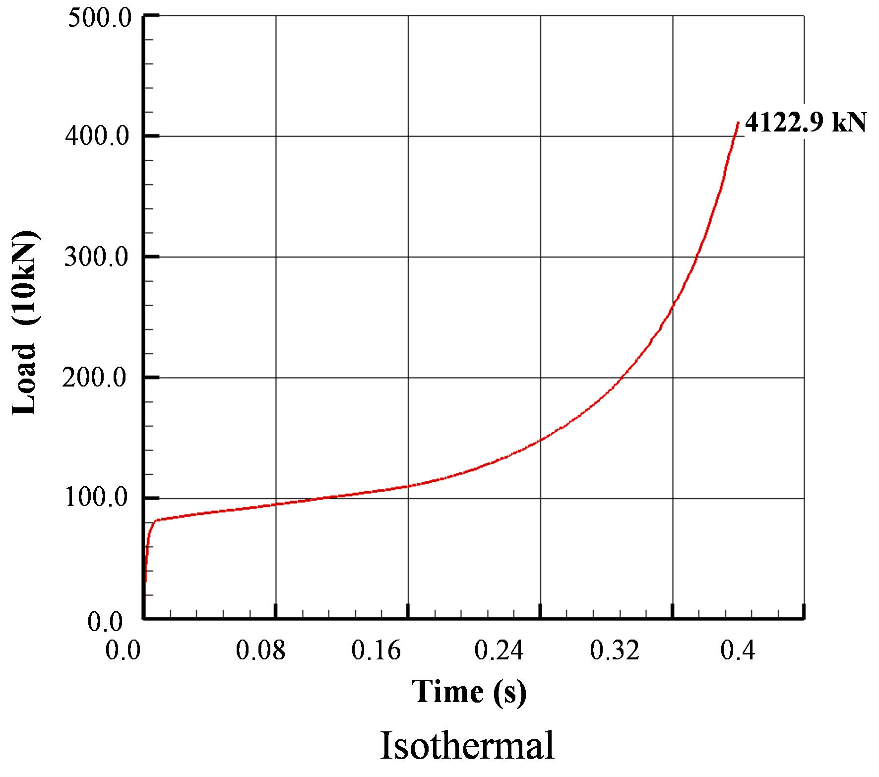
For the purpose of comparing the predicted results of isothermal analysis and non-isothermal analysis, the upsetting process of Figure 12.10(a) (flow stress: Figure 12.10(b)) was analyzed and compared. The main process information is as follows. Material size: (diameter) \(90.0\), (height) \(120.0\text{mm}\); material and flow stress: \(\text{SCr420HB}\), Figure 5.27(b); initial material temperature: \(1150^\circ\text{C}\); friction conditions between material and die: Coulomb friction law (friction coefficient, \(\mu = 0.2\)).
The flow stress curve of Figure 12.10(b) was obtained from compression test results. Non-isothermal analysis was performed with the initial temperature of the die assumed to be \(150^\circ\text{C}\). And the volume-based average temperature (\(1160^\circ\text{C}\)) obtained based on the predicted results of the non-isothermal analysis was calculated, and isothermal analysis was performed using this temperature as the isothermal condition.
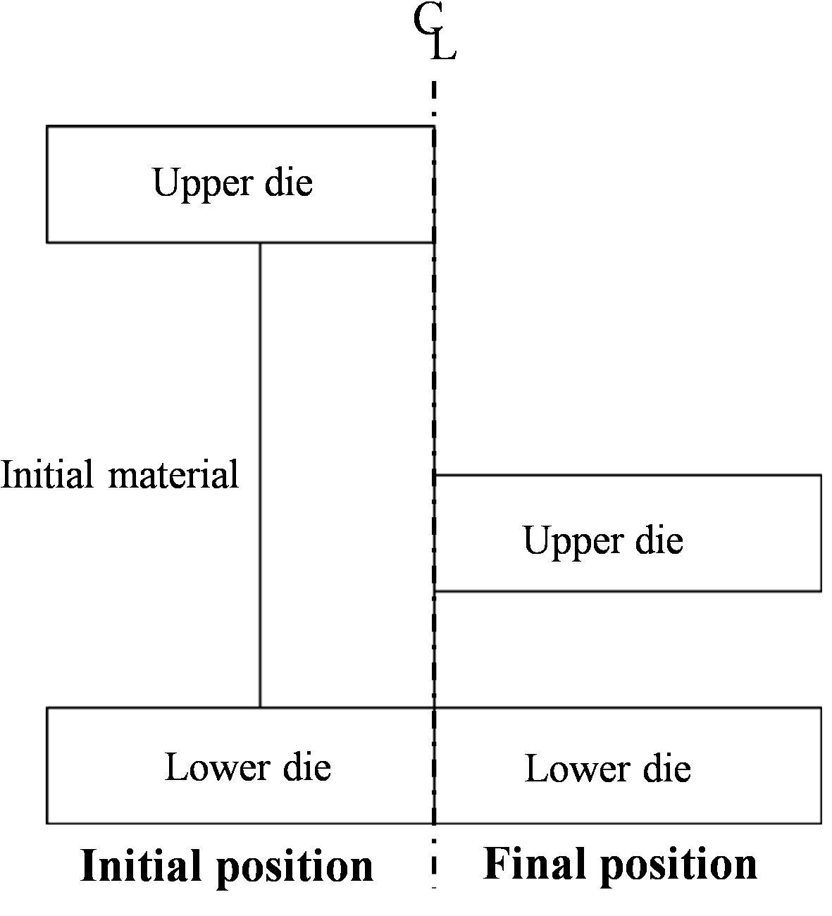
(a) Test process (b) Flow stress
Figure 12.10 Test process information
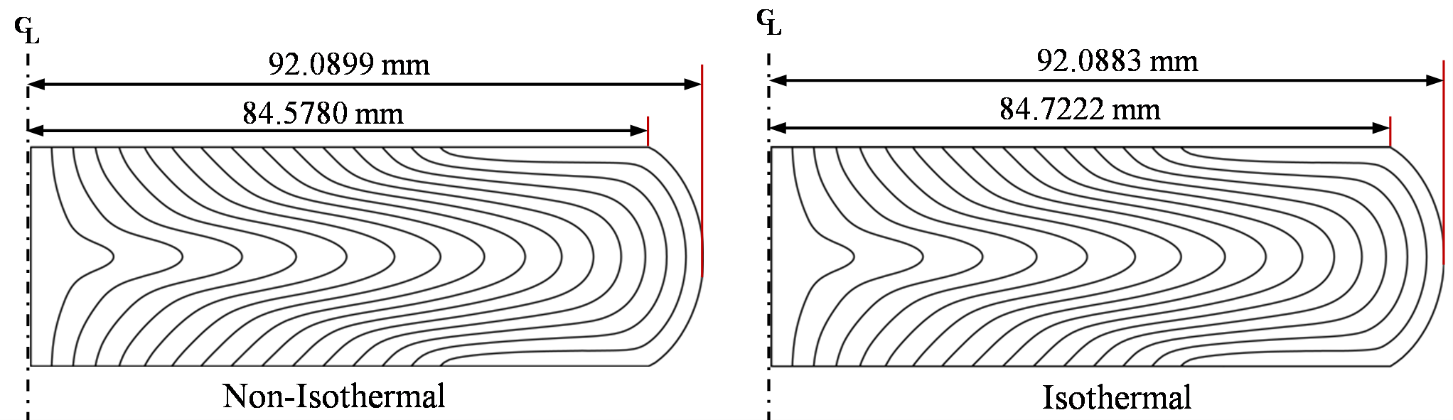
⒜ Deformation
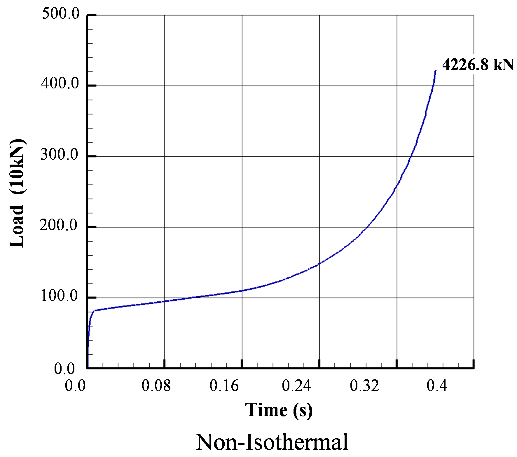
(b) Forming load
Figure 12.11 Comparison of isothermal analysis and non-isothermal analysis of the upsetting process
Figure 12.11 compares the isothermal prediction results and the non-isothermal prediction results for an actual process. Depending on one's viewpoint, there is undoubtedly a non-negligible difference. However, non-isothermal analysis requires thermal boundary conditions whose values can differ greatly depending on the situation, and the data provided in the literature can also show large differences even under the same conditions, so the isothermal prediction results of Figure 12.11 are meaningful in that they provide a reference. To accurately reflect the thermal shock caused by the contact between the die and the material in an actual hot forging process, a dense mesh must be used in the normal direction at the surfaces of the die and material (see the skin element in Section 11.4.1). As shown in Figure 12.13, during the rolling process the rolling roll periodically undergoes sharp temperature rise and cooling only at the roll surface corresponding to 2% or less of the radius, and to solve this problem an ordinary mesh is impossible [11.5]. Forging is basically the same, although to a lesser degree. Nevertheless, the predicted results for the temperature rise due to internal plastic heat are inevitably highly reliable, and can be useful information in the forging of materials that are prone to exposure to hot brittleness (see Section 12.7.2).
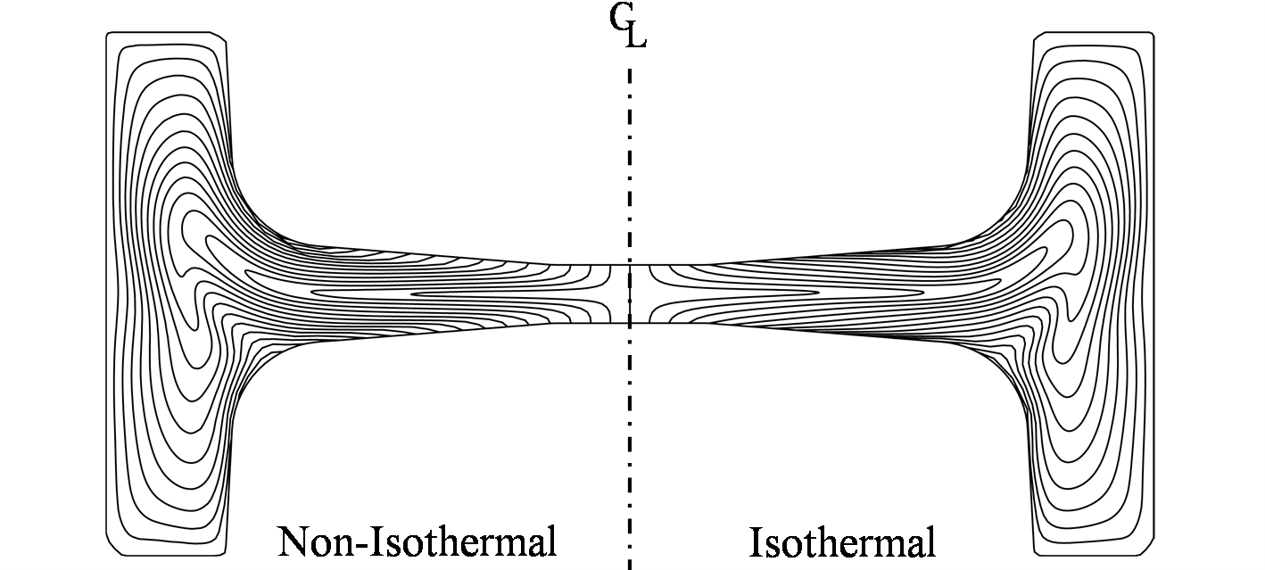
Figure 12.12 Comparison of isothermal analysis and non-isothermal analysis of the first-generation hub bearing forging process
On the other hand, as shown in Figures 12.11 and 12.12, it can be seen that the plastic flow of the non-isothermal analysis is more constrained than that of the isothermal analysis at the die-material contact region. Since this effect can be produced by making the friction coefficient slightly larger than the actual value in the isothermal analysis, if one is interested in predicting the plastic flow lines, isothermal analysis using a modified friction coefficient is also a possible method.
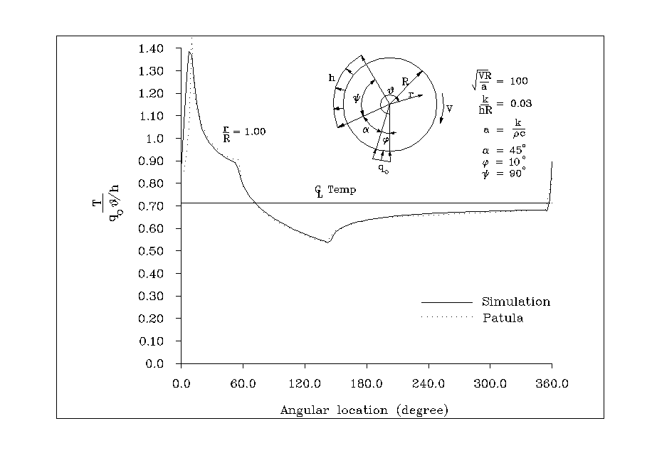
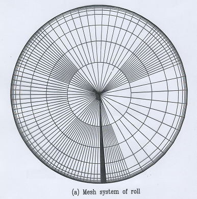
Figure 12.13 Rigid-thermoviscoplastic finite element analysis of the rolling process [11.5]
On the other hand, to analyze the influence of the strain-rate dependence on plastic deformation, assuming the flow stress follows a power law (\(\bar{\sigma} = C\dot{\bar{\varepsilon}}^m\)), isothermal analyses were performed for conditions such as the strain-rate dependence exponent $m =0.05, 0.1, 0.15 etc., and for the two cases of high and low speed, and the results are shown in Figures 12.14 and 12.15. The conditions used to perform this analysis are as follows. Friction coefficient: 0.2; speed: low speed (50 mm/s), high speed (250 mm/s); material size: radius 45.0 mm, height 120.0 mm.
As shown in Figure 12.15, both at low and high speed the deformed shape shows a non-negligible difference depending on the strain-rate dependence, but this does not govern the analysis results. In contrast, as shown in Figure 12.16, when the high-temperature strength coefficient is assumed to be equal to 1.0, the difference in forming load according to the strain-rate exponent appeared large compared to the deformation, both at low and high speed, and in the high-speed case the difference is particularly pronounced.
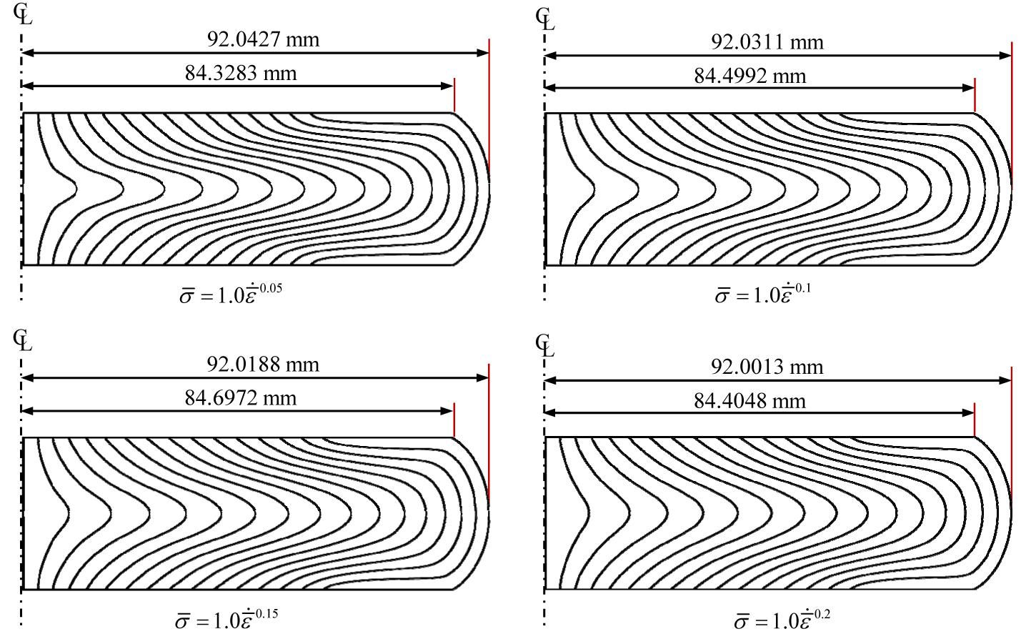
⒜ At low speed (speed = 50 mm/s)
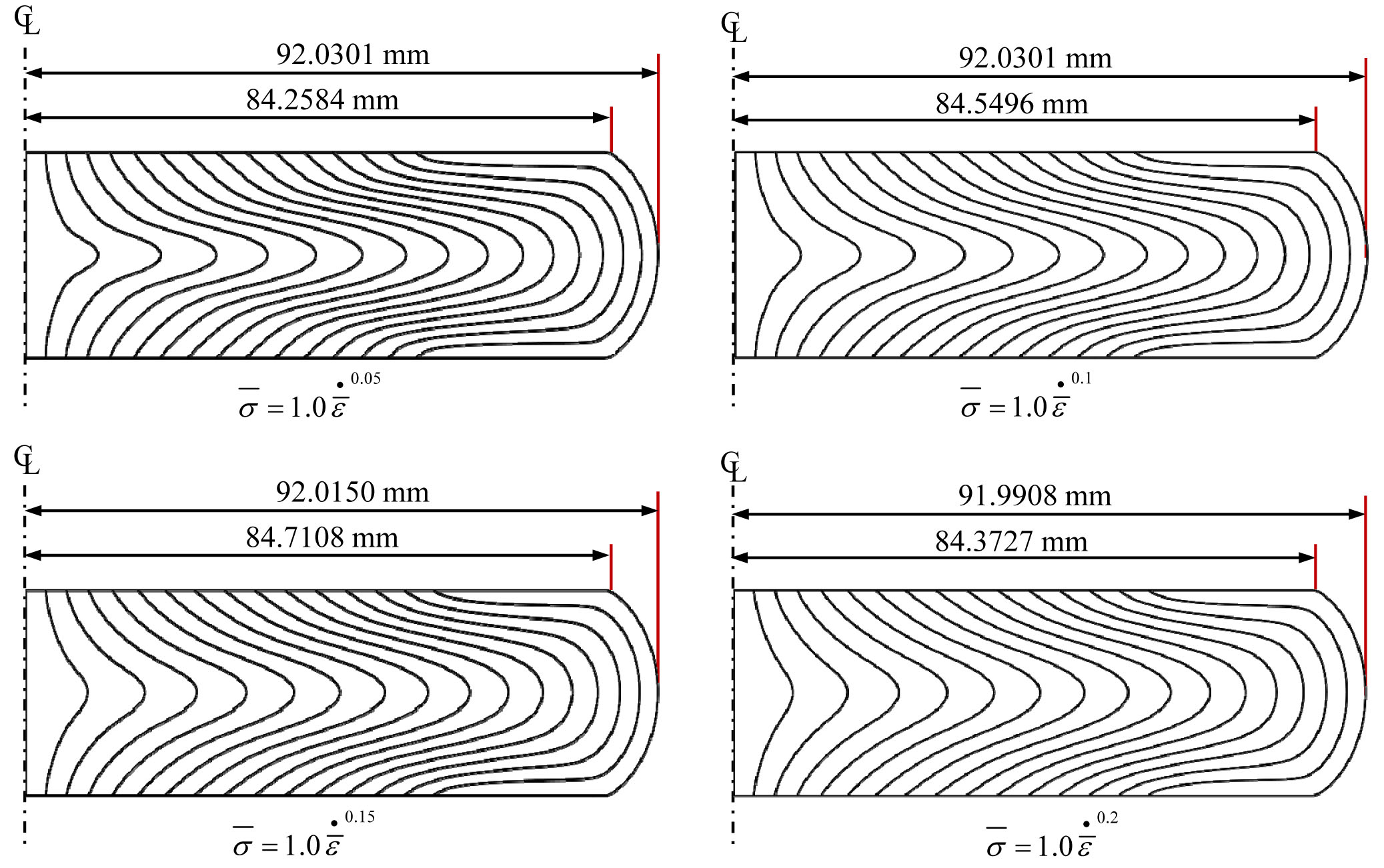
⒝ At high speed (speed = 250mm/s)
Figure 12.15 Strain-rate dependence exponent
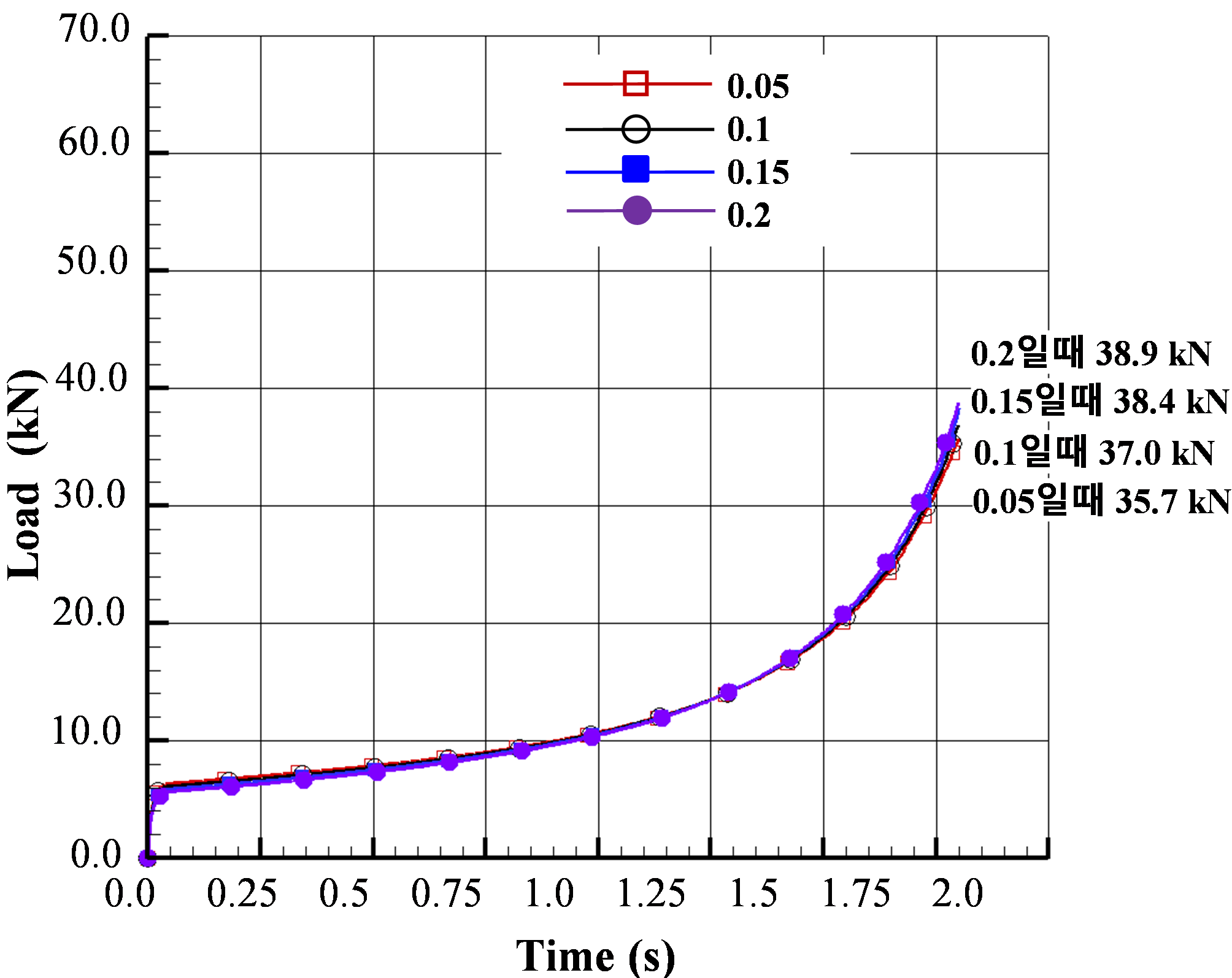
⒜ At low speed (speed = 50 mm/s)
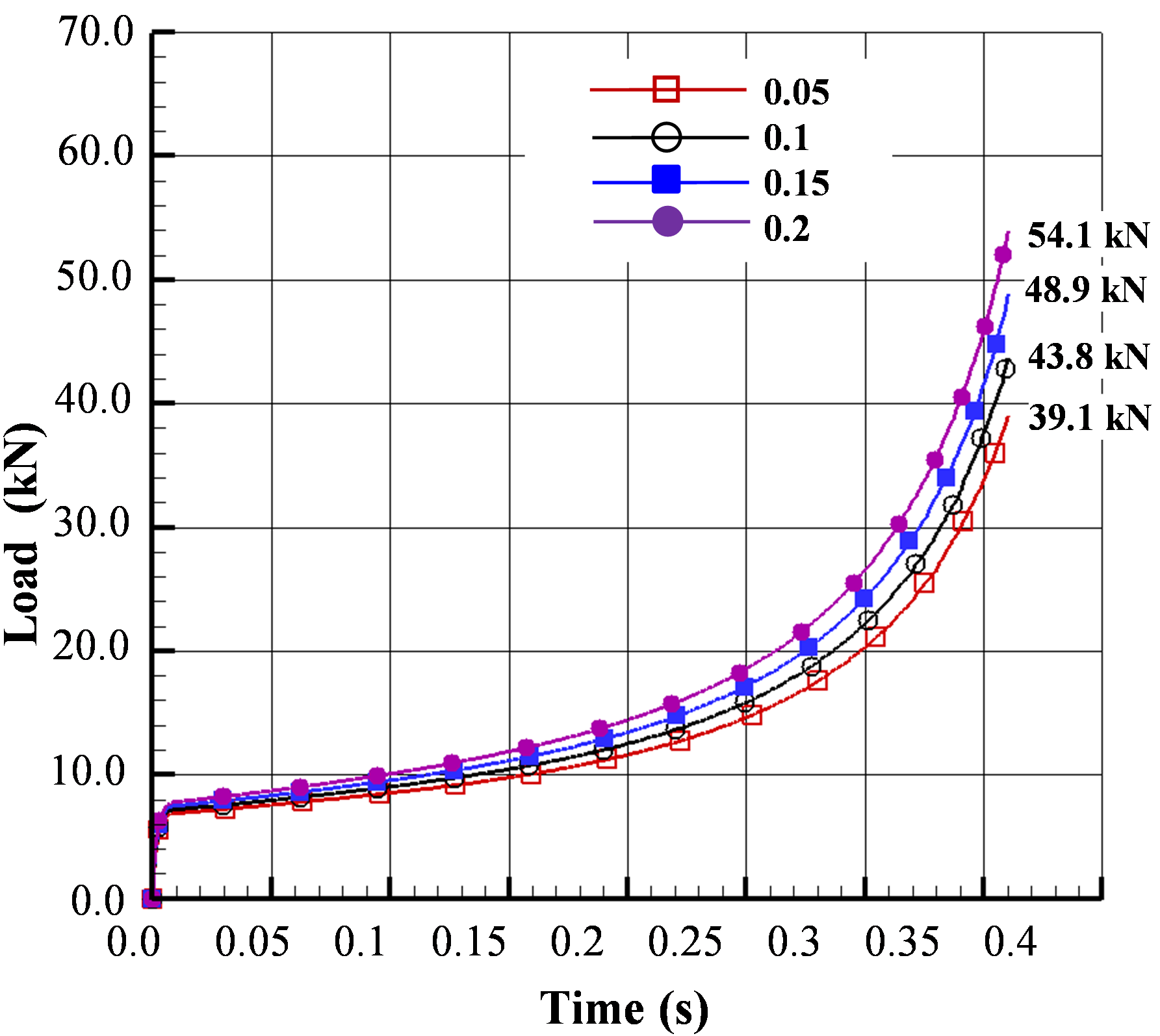
⒝ At high speed (speed = 250mm/s)
Figure 12.16 Strain-rate dependence exponent and forming load
In conclusion, the validity of the analysis results varies greatly depending on what one wishes to obtain. If one wishes to see the plastic flow lines, i.e., the flow lines and the approximate relative values of the load, there is no need to perform non-isothermal analysis, and the speed can be taken as an average value. This result is meaningful in its own way, because it provides a relatively stable theoretical solution. In particular, when conceptually designing a certain process or improving it based on the analysis results of an existing process, simplified flow stress and isothermal analysis are effective. When the theory becomes complex and the number of input variables increases, the accuracy is more likely to increase, but the opposite possibility always exists as well. However, for metallurgical predictions including microstructure, the use of a more scientific and higher-degree-of-freedom flow stress that includes recrystallization is unavoidable.
12.3.3.2 High-Temperature Flow Stress Model
Compared to room temperature, obtaining the flow stress in the high-temperature state involves greater difficulty. It is true that the high-temperature flow stress of a material is difficult to obtain and not easy to find in the literature. The reason is that the material is deformed in an extreme state of high temperature and high pressure. Fortunately, even using flow-stress-related information obtained from limited data, the plastic flow analysis results are meaningful.
The flow stress of a thermoviscoplastic material for reflecting the characteristics of metal materials at high temperature is often formulated and used as follows.
Here, \(n\), \(m\), etc., are called the strain-hardening exponent and the strain-rate dependence exponent (strain rate dependence), respectively, and together with the high-temperature strength coefficient \(C\), are functions of temperature and strain, etc.
In practice, obtaining the material information of Eq. (12.10) involves much difficulty. This is because the high-temperature characteristics of the material are complex and measurement of the material information is not easy in the extreme situation of high temperature and high pressure. For this reason, the material information obtainable from references is also limited. Empirically, the results of isothermal analysis performed using a strain-rate-dependent material reflect actual phenomena relatively well. The behavior characteristic curve of a strain-rate-dependent material is as shown in Figure 4.5, and the flow stress function on the left side of this curve is often expressed by the following mathematical model.
(4) Cingara high-temperature strain-hardening model
(5) Voce model
Here,
(6) Misaka-Yoshimoto model
(7) Ebrahimi et al. model
Here, the coefficients are obtained using a graphical method.
(8) Improved Ebrahimi et al. model
Precewik bilinear function:
Closed-form function:
Among the flow stress model formulas introduced above, the variables that are not defined are material constants and belong to the material properties. The material properties are obtained through material tests including tensile tests, compression tests, and torsion tests, together with curve fitting and optimization using mathematical models. Among the formulas above, the improved Ebrahimi et al. model allows the material constants to be obtained under the systematic support of an optimization-based material constant acquisition program. The details of this are described in Section 12.6. Meanwhile, the flow stress is influenced not only by strain, temperature, and strain rate but also by other factors. Representative ones are the damage, recrystallization, and grain size.
12.4 Method for Obtaining High-Strain Flow Stress by Tensile Testing
The tensile test provides engineers with much information about the mechanical properties of a material. The elastic modulus, yield stress, tensile strength, elongation, and the true strain–true stress relationship up to the onset of necking are representative mechanical properties of a material obtainable by tensile testing. In addition, the tensile test gives engineers much intuition about materials. In this respect, understanding the mechanical phenomena occurring during the tensile test is important.
The characteristic feature of the tensile test is necking. Understanding the necking phenomenon is important for understanding the macroscopic characteristics of the material occurring in the tensile test. In particular, accurate analysis of the necking phenomenon using the finite element method not only helps in understanding and applying the mechanical phenomena that occur thereafter, but also helps in evaluating the suitability of the analysis program, in the correct setting of analysis conditions, and in advancing the utilization technology.
Analytical research on tensile testing using the finite element method has not been carried out much relative to its importance. A survey of the relevant literature [12.3, 12.5] shows that it is divided into cases such as: modeling including the grips but without imposing an initial defect; modeling the rectangular region between the gauge points of the specimen but imposing an initial defect or constraining the displacement of one end; and artificially making the strain maximum at the necking region. As for the material shape, round bars and sheets or square-section bars have been mainly studied. In some studies the material was formulated as rigid-plastic, and in the other studies the material was formulated as elastoplastic or viscoelastoplastic, and many studies used commercial programs.
If Hollomon's flow stress model equation is used, theoretically necking occurs when the true strain becomes equal to the strain-hardening exponent, and at this point the maximum load must act (called the Considère condition). Many researchers were interested in predicting the onset of necking, but a study reporting that this condition is accurately satisfied was published in 2007 [12.5].
Necking occurs because the reduction in structural strength of the tensile specimen due to the decrease in cross-sectional area exceeds the increase in the material's flow stress due to strain hardening, so it is an inherent property of the material. Therefore, the artificial condition settings used in previous studies are not valid. The authors' research group [12.5] accurately predicted the onset of necking in the tensile test of a round-section bar using a perfect model of the complete tensile test analysis of a simple bar modeling the gauge section, and the results are shown in Figure 12.17. The material used in the experiment in the figure is SWCH10A, pretreated for the purpose of automatic multi-stage cold forging. The flow stress used in the analysis was expressed by the Hollomon model formula, and to satisfy the Considère condition, the true strain at the necking point was used as the strain-hardening exponent. As a result, the necking point was accurately predicted, but as shown in Figure 12.17, after the necking point the experimental results and predicted results show a large difference. This indicates the limitation of the Hollomon formula.
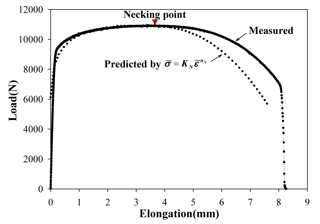
Figure 12.17 Comparison of the analysis results and experimental results of the tensile test using the Hollomon model formula
On the other hand, during a tensile test the material just before fracture reaches a high-strain state in the necking region. Taking this point together with the problems inherent in the Hollomon flow stress equation, the authors' research group [12.6] presented a method that accurately predicts the tensile test from an engineering viewpoint. In this method, the flow stress is formulated by the following modified Hollomon model flow stress equation.
Here, the strength coefficient K is formulated as a function of strain. This method has the advantage of being able to obtain true strain–true stress information even for high strains (for SCM435, up to about 1.5 as shown in Figure 12.19), and analyzing the tensile test using the rigid-plastic finite element method with the obtained stress-strain curve can accurately predict the entire tensile test. Based on this method, AFDEX/MAT was developed for the purpose of obtaining the flow stress of materials at room temperature. The detailed approach is replaced by the relevant reference [12.6].
This method is based on a sequential approach, and as shown in Figure 12.18(b), it can be seen that there is little change after three iterations. The flow stress curve obtained by four iterations expresses the flow stress up to a maximum strain of about 1.1, and as a result of analyzing the tensile test using this curve, the maximum error between the experimental results and predicted results was found to be 0.3% or less, as shown in Figure 12.18(b). This result implies that it is no exaggeration to say that the predicted flow stress is, from an engineering standpoint, the correct answer.
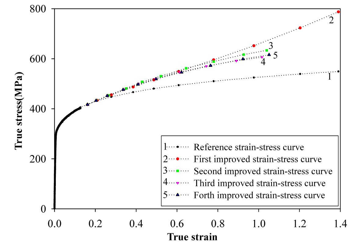
⒜ Sequential improvement of the true strain–true stress curve
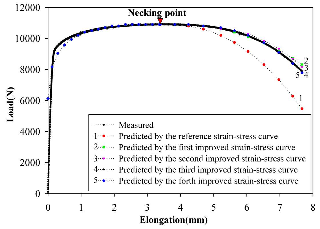
⒝ Improvement process of the predicted elongation–tensile force curve
Figure 12.18 Acquisition of flow stress
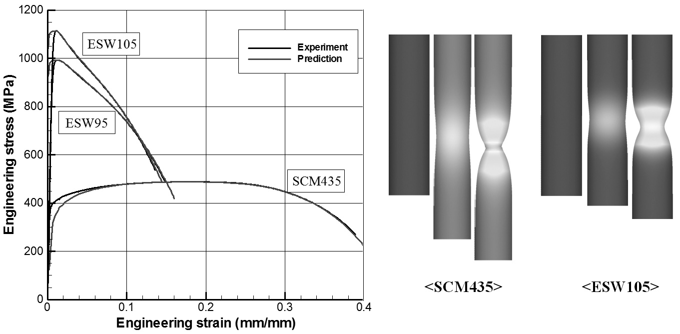
Here, the results of applying it to SCM435, a typical strain-hardening material, and to ESW95 and ESW105, high-strength materials with very small strain-hardening capacity, are introduced. The results of applying AFDEX/MAT are summarized in Figures 12.19 and 12.20. Figure 12.19⒜ shows the tensile test results, and Figure 12.19⒝ shows the flow stress curves obtained from these tensile test results using AFDEX/MAT. Figure 12.20⒜ shows the tensile test analysis results, and Figure 12.20⒝ shows the deformation history obtained from the tensile test analysis results. It can be confirmed that the experimental results and analysis results of the tensile test agree well in the plastic region. For reference, the flow stress obtained through a simple compression test is reliable at strains of 0.5 or less, and at strains above that, reliability inevitably decreases due to the barreling phenomenon.
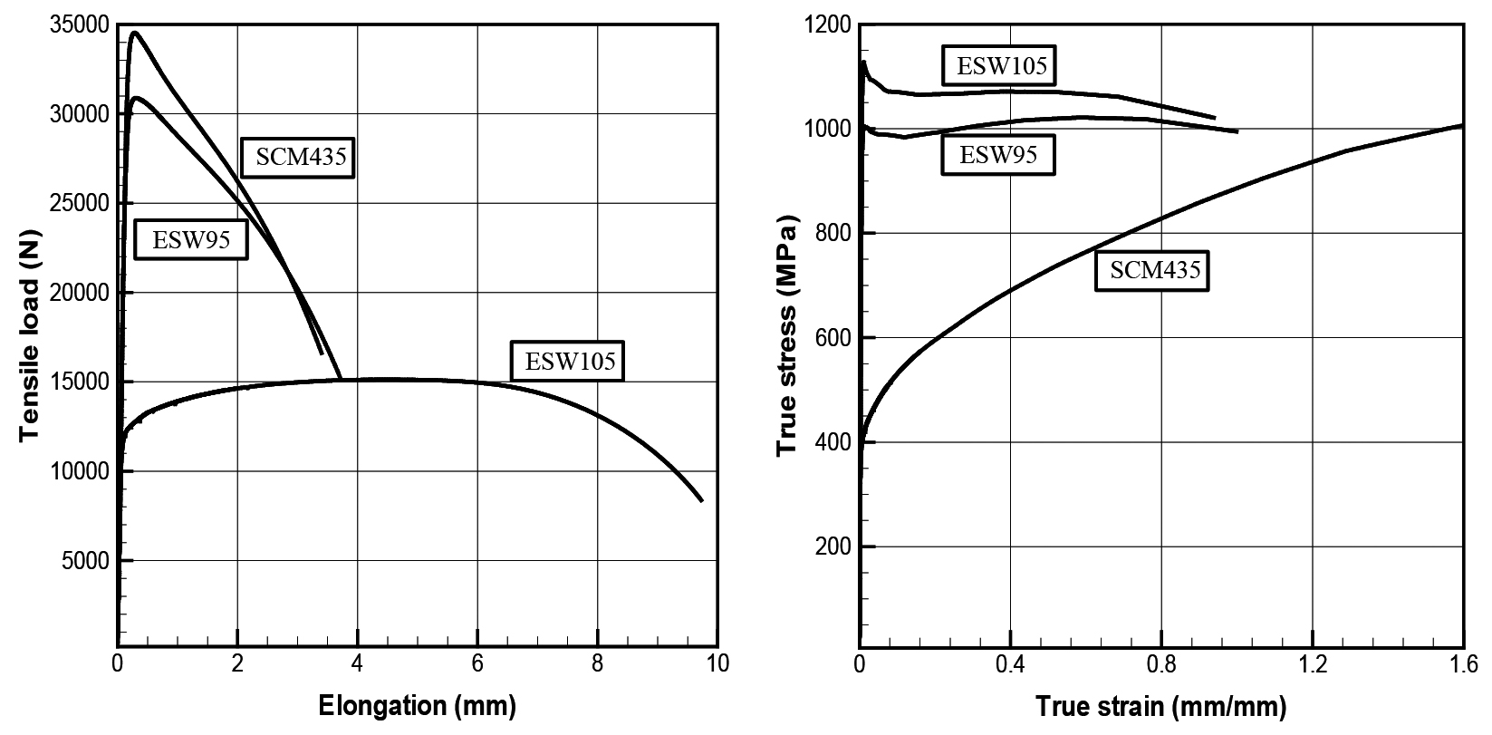
(a) Tensile test results (b) True stress–true strain curve
Figure 12.19 Acquisition of material flow stress using AFDEX/MAT
(a) Comparison of experimental results and predicted results (b) Deformation history of the tensile test
A notable point in the flow stress curves is that for SCM435, the flow stress was obtained for effective strains up to 1.6. And it shows a phenomenon in which the strain-hardening capacity decreases as the strain increases. This implies that the strain-hardening capacity of a material that has been deformed through processes such as upsetting or drawing decreases. Therefore, securing and utilizing the initial state of the material, i.e., the initial strain, is important in metal forming simulations.
12.5 Acquisition of High-Temperature Flow Stress
12.5.1 Power-Law Flow Stress Model
12.5.1.1 Alloy Steel
In this section, the quantification and utilization method of the power-law flow stress model are explained for STB2, a type of alloy steel.
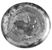
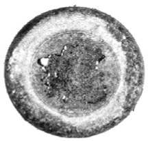
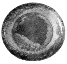
The easy method for obtaining the flow stress of a material in the high-temperature state is, of course, the compression test. The high-temperature compression test of STB2 was conducted for a total of 24 types: 6 sampling temperatures (900, 1000, 1100, 1150, 1200, 1250) and 4 sampling strain rates (1, 5, 10, 50/s). Figure 12.21 shows the specimens after the compression test. These are the shapes of specimens obtained by high-temperature compression testing at a constant strain rate (10/s) up to a compression ratio of 75%. From this figure, it can be confirmed that cracks occurred along with barreling on the side of the specimen tested at 1250°C. This phenomenon is consistent with the result of the sharp drop in the reduction of area during the tensile test in Figure 22.4⒜.
⒜1100℃
⒝1150℃
⒞1200℃
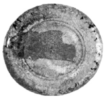
(d)1250℃
Figure 12.21 High-temperature compression specimens
Figures 12.22 and 12.23 are the high-temperature compression test results. Figure 12.22 shows the stress-strain curves obtained by conducting high-temperature compression tests at various temperatures under a constant strain rate (10/s). It can be seen that the stress-strain curves obtained from the high-temperature compression test differ from the stress-strain curves at room temperature. As shown in the figure, it can be seen that the flow stress decreases as the temperature rises.
Figure 12.23 shows the stress-strain curves for various strain rates (1, 5, 10, 50/s) at a constant temperature (1150℃). As shown in the figure, it can be seen that the flow stress increases as the strain rate increases. As for the shape of the stress-strain curve, below the peak strain the flow stress increases sharply as the strain increases, and reaches the maximum stress at the peak strain. After that, the flow stress decreases at a relatively large rate, and after a certain deformation the rate of decrease of the flow stress becomes small or tends to maintain a steady state. The stress-strain curve shows the form of a typical dynamic recrystallization curve.
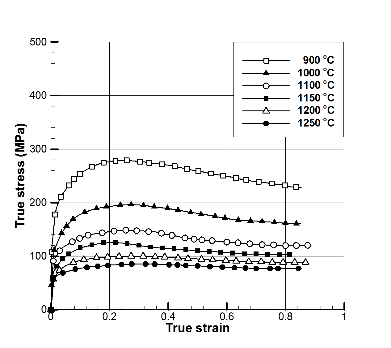
Figure 12.22 True stress–true strain curves at a strain rate of 10/s
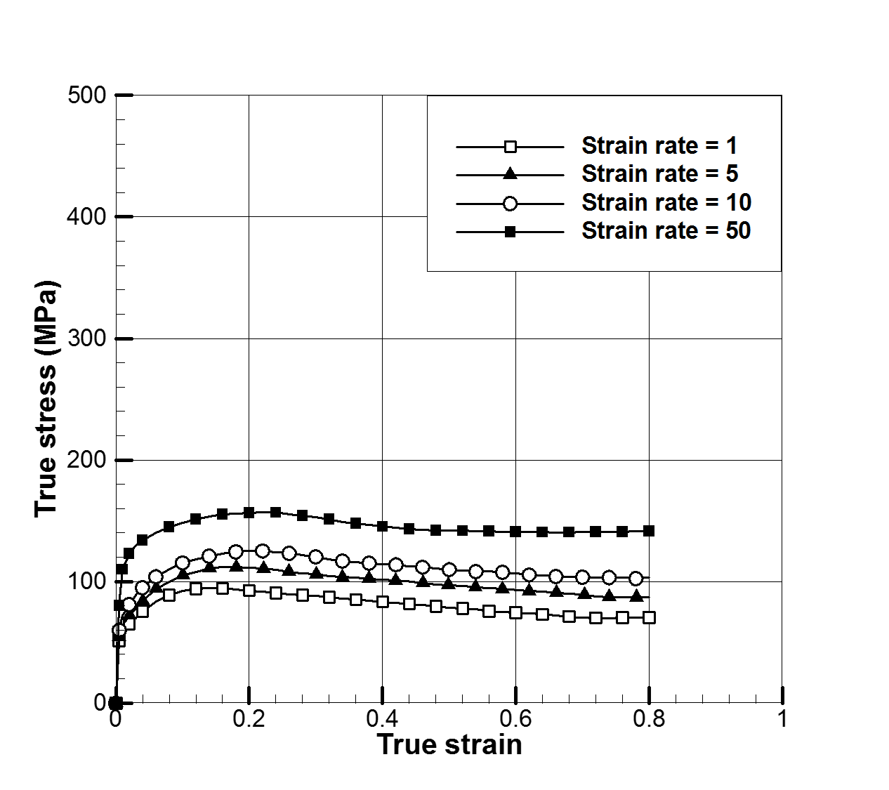
Figure 12.23 True stress–true strain curves at a constant temperature (1150 ℃)
In the compression test, the flow stress curve shows various patterns as the strain increases. A critical strain or peak strain is required to cause recrystallization, and up to this point strain-hardening capacity is exhibited. And once this critical value is exceeded, a softening phenomenon due to the decrease in flow stress caused by recrystallization generally occurs. If the specimen is deformed at high speed, the flow stress tends to increase continuously because the rate of strain hardening is large compared to the recrystallization rate. If deformed at low speed, strain hardening and softening due to recrystallization repeat, so oscillation of the flow stress may occur.
ㄹThe problem is how to formulate and utilize these results. These curves are often fitted by Eq. (12.12). In general, the influence of the strain-hardening exponent is neglected. Instead, \(C\) and \(m\) are assumed to be functions of temperature and strain. For example, in Figure 12.23, when the temperature of the STB2 material is 1150℃ and the strain is 0.3, the strain rate and flow stress are as shown in Table 12-1. The \(C\) and \(m\) values that best reflect these values can be obtained by the least-squares method, but the \(C\) and \(m\) values can also be easily obtained by hand calculation using the following approximate method. By exactly satisfying the case where the strain rate is 1.0, \(C\) = 91.0 is obtained, and if the \(m\) values that exactly satisfy the cases where the strain rate is 10.0, 20.0, and 30.0 are obtained, they become 0.095, 0.120, and 0.133, respectively; taking the average of the \(m\) values gives \(m\) = 0.116. As shown in Figure 12.24, the \(C\) = 91.0 MPa and \(m\) = 0.116 thus obtained reflect the test results relatively well.
[Table 12-1] Strain rate and flow stress at sampling points
| Strain rate | Flow stress | \(C\) | \(m\) |
|---|---|---|---|
| 1.0 | 91.0 | 91.0 | |
| 5.0 | 106.0 | 91.0 | 0.095 |
| 10.0 | 120.0 | 91.0 | 0.120 |
| 50.0 | 153.0 | 91.0 | 0.133 |
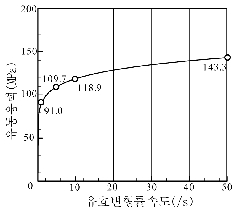
Figure 12.24 Comparison of test data and the approximate flow stress–effective strain rate curve
On the other hand, in the compression test results, reliability inevitably decreases toward higher strains because of the barreling phenomenon. Of course, at high temperature, due to the occurrence of recrystallization, high strain cannot practically be maintained. Generally, this critical value is regarded as around 0.7. Therefore, for strains larger than this value, it is common to calculate the flow stress using this critical value. Of course, there can be a method of obtaining the residual strain by coupling recrystallization, etc., during the analysis, but to make this technique practical, additional research must be carried out, and specialized knowledge is required of the user as well.
Table 12-2 summarizes the high-temperature strength coefficient \(C\) and the strain-rate dependence exponent \(m\) obtained using the least-squares method. This point-cloud data is used to calculate the \(C\) and \(m\) values corresponding to an arbitrary temperature and strain during finite element analysis by interpolation.
[Table 12-2] High-temperature strength coefficient \(C\) [MPa] and strain-rate dependence exponent \(m\)
| Temperature | 900 | 900 | 1000 | 1000 | 1150 | 1150 |
|---|---|---|---|---|---|---|
| Strain | \(C\) | \(m\) | \(C\) | \(m\) | \(C\) | \(m\) |
| 0.1 | 182.2 | 0.151 | 142.0 | 142.0 | 89.05 | 0.123 |
| 0.3 | 190.2 | 0.151 | 151.6 | 0.126 | 88.40 | 0.136 |
| 0.5 | 176.6 | 0.154 | 138.8 | 0.123 | 78.20 | 0.149 |
| 0.7 | 16.85 | 0.145 | 126.0 | 0.130 | 69.01 | 0.178 |
12.5.1.2 Aluminum Alloy
In this section, a case study of the quantification of the power-law flow stress model for Al6061, an aluminum alloy, is briefly introduced. The diameter and height of the high-temperature compression test specimen used are 8.0 mm and 12.0 mm, respectively. As test conditions, the compression ratio is 50–60%, the strain rate is 0.1–20.0/s, and the test temperature is 300–550℃.
Figure 11.25 shows the flow stress–strain curves obtained from the high-temperature compression test. From the curves in Figure 11.25, it can be seen that as the temperature increases, the flow stress decreases, and as the strain rate increases, the flow stress increases. And it can also be seen that below a certain strain, strain has a relatively large influence on the flow stress, but after reaching the strain at which the flow stress is maximum, i.e., the peak strain, and reaching a certain strain, the increase in strain does not have a large influence on the change in flow stress. The stress that reaches this constant value is called the steady-state stress. This is because, after the peak strain, recrystallization occurs and relaxes strain hardening, thereby impeding the increase in flow stress. This pattern also appears in steel, and the difference between steel and aluminum is only a difference in the magnitude of the values. If two different materials showed identical flow stress characteristics, they would be said to be mechanically identical. However, if the thermal characteristics and fracture characteristics of these two materials differ, the analysis results differ, or the meaning of those results becomes different.
In general, the flow stress function for reflecting the characteristics of a material heated to high temperature, i.e., a strain-rate-dependent material, is expressed by Eq. (12.12) in which strain hardening is neglected. That is, \(\bar{\sigma} = C \dot{\bar{\varepsilon}}^m\). Here, \(C\) is the high-temperature strength coefficient, and \(m\) is the strain-rate dependence exponent. Ultimately, different materials mean that these values are different.
[Table 12-3] High-temperature strength coefficient \(C\) [MPa] and strain-rate dependence exponent \(m\)
| Temperature | \multicolumn{2}{c | }{300} | \multicolumn{2}{c | }{350} | \multicolumn{2}{c | }{350} | \multicolumn{2}{c | }{450} | \multicolumn{2}{c | }{500} | \multicolumn{2}{c | }{550} |
|---|---|---|---|---|---|---|---|---|---|---|---|---|
| Strain | \(C\) | \(m\) | \(C\) | \(m\) | \(C\) | \(m\) | \(C\) | \(m\) | \(C\) | \(m\) | \(C\) | \(m\) |
| 0.1 | 84.98 | 0.045 | 64.37 | 0.054 | 49.33 | 0.063 | 41.51 | 0.105 | 36.82 | 0.109 | 31.41 | 0.118 |
| 0.2 | 87.69 | 0.044 | 66.60 | 0.058 | 50.60 | 0.073 | 41.22 | 0.103 | 37.10 | 0.103 | 30.90 | 0.121 |
| 0.3 | 89.26 | 0.038 | 65.92 | 0.065 | 50.37 | 0.070 | 41.92 | 0.100 | 36.17 | 0.103 | 29.76 | 0.122 |
| 0.4 | 89.34 | 0.039 | 65.36 | 0.055 | 49.74 | 0.067 | 40.09 | 0.104 | 35.54 | 0.099 | 29.23 | 0.109 |
Table 12-3 summarizes the results of obtaining the strength coefficient \(C\) and strain-rate dependence \(m\) of Al6061 for each strain and temperature by the curve-fitting method using the information of Figure 12.25 obtained from the high-temperature compression test and the mathematical model of Eq. (12.12). Within the range of strain rates conducted in this test, when the strain is 0.4 or more, the material constants are not greatly influenced by strain.
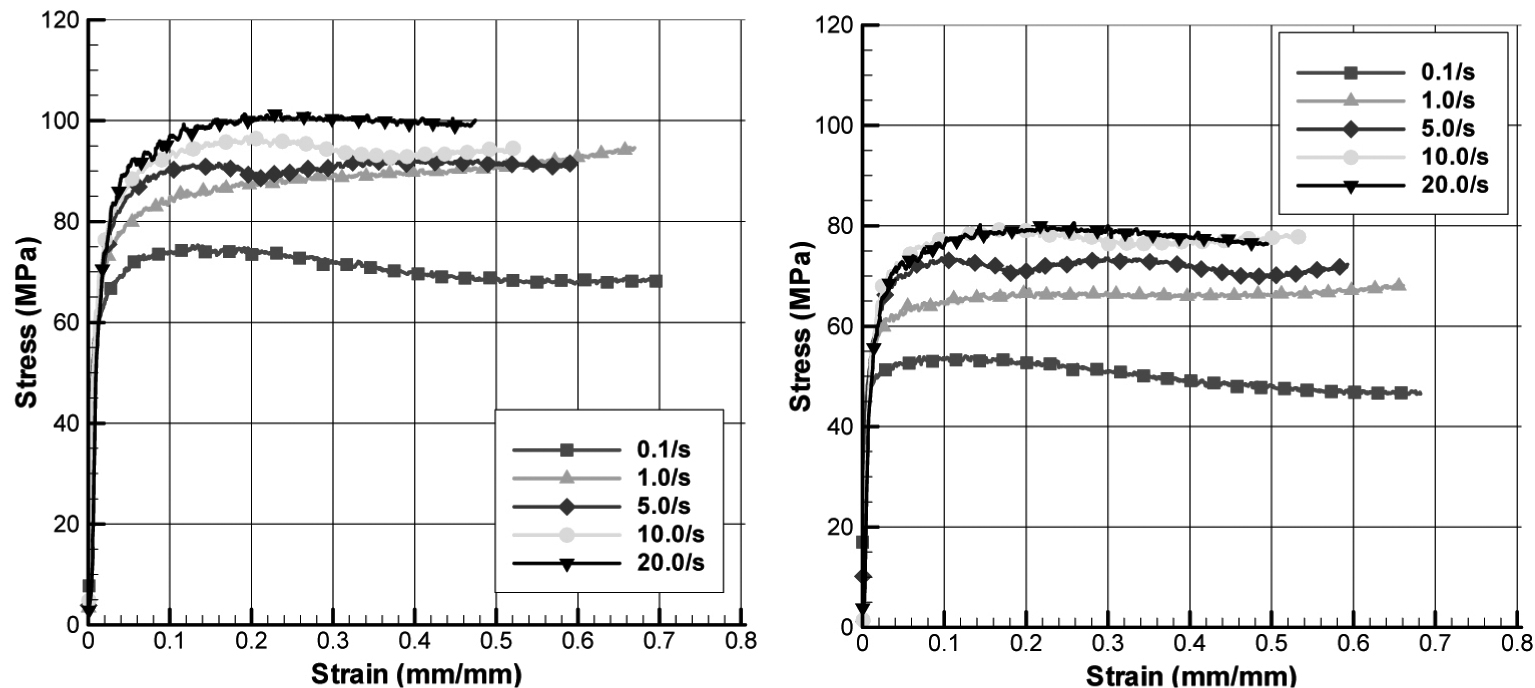
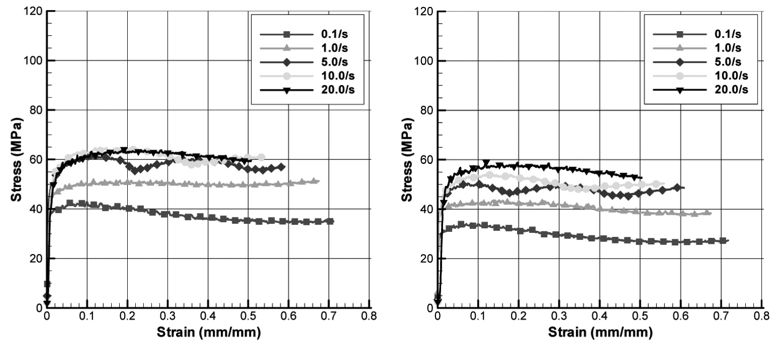
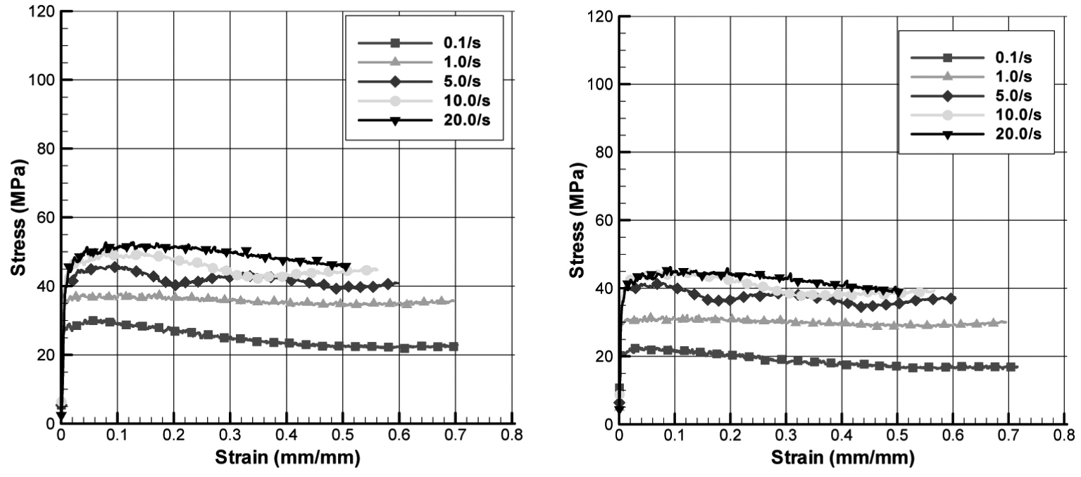
Figure 12.25 Flow stress of Al6061 according to temperature and strain rate
12.5.2 Phenomenological Model Emphasizing Softening Due to Recrystallization
12.5.2.1 Flow Stress Model Based on a Metallurgical Background
Figure 12.26 is a typical example of a flow stress curve in which the softening phenomenon has occurred. Up to the peak strain it exhibits strain-hardening characteristics, and softening occurs due to recrystallization; when a certain strain, i.e., \(\varepsilon_s\), is reached, it reaches a steady state where strain hardening and this softening are balanced.
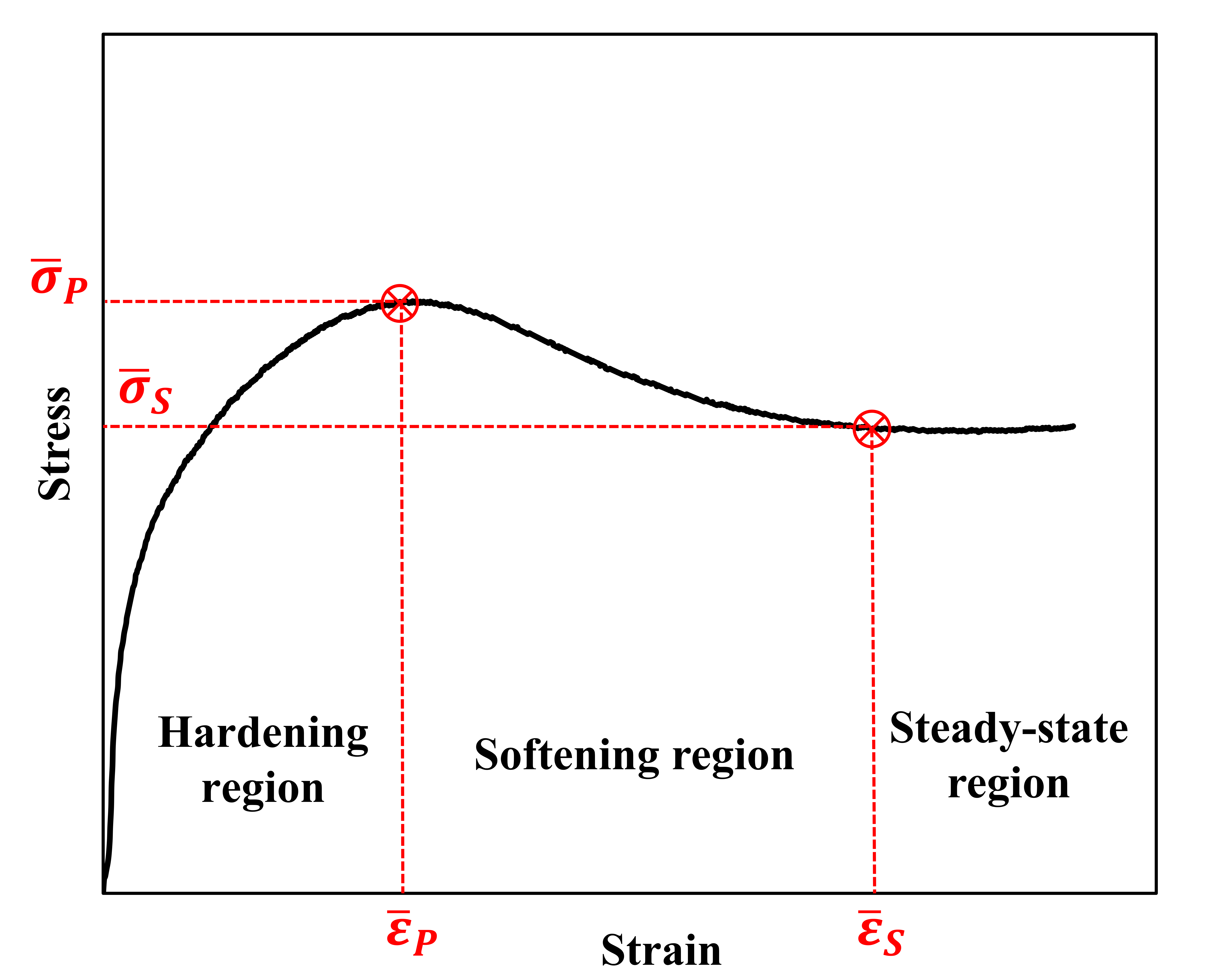
Figure 12.26 Conceptual diagram of a high-temperature flow stress curve
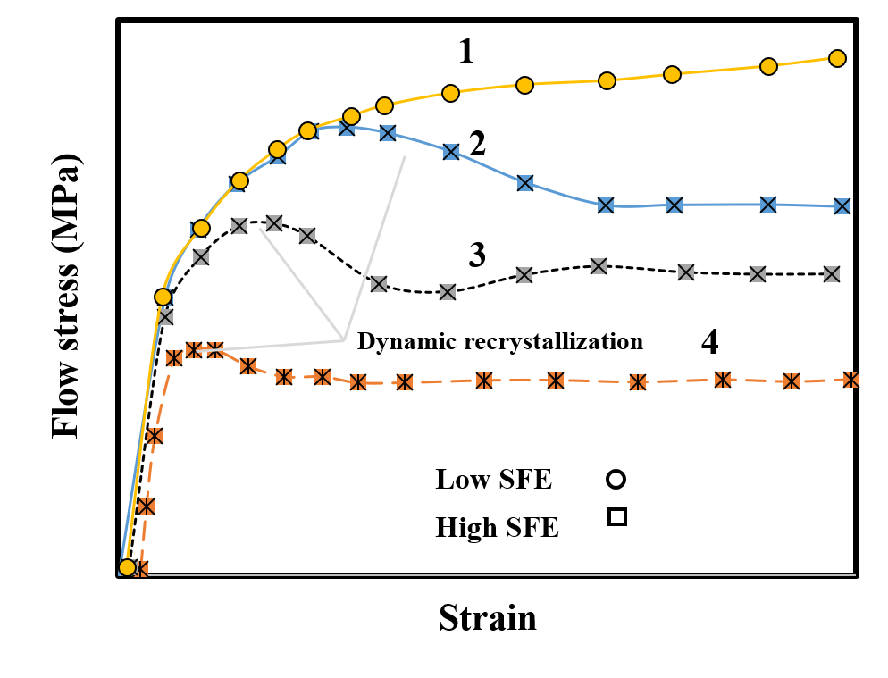
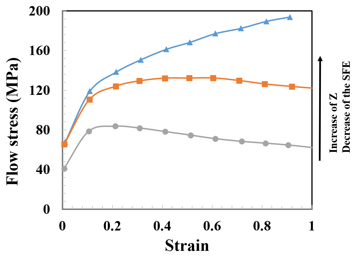
It is reflected by the curve, i.e., the relationship between flow stress and strain. A typical example of the material's response to deformation is shown in Figure 12.27⒜. The form of this response depends on the stacking fault energy (SFE) of the material. In Figure 12.27⒜, curves 1 and 2 represent the responses of low-SFE and high-SFE materials, respectively.
⒜ Typical plastic flow behavior
⒝ Typical mathematical model of flow stress
Figure 12.27 Behavior characteristics and mathematical model of flow stress
In the case of a low-SFE material, low energy is accumulated in the material, and dynamic recrystallization (DRX) is not initiated. The material's response should be regarded as a competition between hardening and softening. That is, the hardening phenomenon and the softening phenomenon are not one-sided. In the case of a high-SFE material, the high energy stored in the material leads to the initial formation of DRX. In Figure 12.27⒜, curves 3 and 4 represent the deformation characteristics of the material at low Zener-Hollomon coefficients, respectively. The Zener-Hollomon coefficient, or coefficient, is defined by the following equation.
Here, the material constants and state variables used together with the strain rate are as follows. [ R, \quad T, \quad Q_d ] are the gas constant, temperature, and deformation activation energy, respectively. The deformation activation energy is a material constant.
Traditional flow stress models widely used for the purpose of metal forming process analysis yield relatively satisfactory results when the deformation conditions are somewhat monotonic. Hollomon is a representative researcher for expressing the flow stress in terms of the state variables of the process. He proposed the following power-law model.
The variable symbols used here are as follows, respectively. [ \varepsilon, \quad n, \quad k ] are strain, strain-hardening exponent, and strength coefficient, respectively. To reflect the influence of temperature, the following equation has been proposed by adding a power-law function of strain rate and an Arrhenius term for temperature [12.7].
Sellars and Teggart [12.8] supplemented the shortcomings of Eq. (12.26) and proposed the following flow stress model using the following coefficient and the \(\sinh^{-1}\) function. [ Z ] This is called the Zener-Hollomon coefficient, and the mathematical model is as follows.
The foregoing equation is suitable for expressing the flow stress when the Zener-Hollomon coefficient is large. However, when this coefficient is small, softening of the material due to DRX occurs, and this has an important influence on the deformation characteristics. [ Z ] In addition to the coefficient, the SFE is a main variable that influences DRX. If the SFE is small, a large strain must be accumulated to cause DRX.
The flow stress of the foregoing equation is often used in conjunction with the following Voce model to explain strain hardening, softening, DRX, etc.
The independent symbols used here are as follows. [ \bar{\sigma}p, \quad \bar{\sigma}_o, \quad \bar{\sigma}_s, \quad X, \quad B ] are the peak stress, the flow stress for explaining strain hardening only (initial stress), the steady-state stress, the recrystallized volume fraction, the strain, and a material constant, respectively. Many of the variables are functions of Z, and their relations are as follows.}, \quad \bar{\varepsilon
The constant symbols used here are as follows. [ c_o, \quad d_o, \quad c_1, \quad c_2, \quad e_o, \quad e_1, \quad e_2, \quad f_o, \quad f_1, \quad f_2, \quad g_o, \quad g_1, \quad g_2 ] These are material constants that must be obtained for each material.
Therefore, the Voce model is attractive in that it emphasizes the microstructural evolution phenomenon and expresses the flow stress as a function of strain, strain rate, temperature, etc., but unfortunately there is no well-established method for easily obtaining these material constants.
Figure 12.28 shows a case study of applying the Voce flow stress model to the alloy steel 20MoCrS4. Although it contains errors within a generally acceptable range over the entire strain range, it can be confirmed that the results are generally satisfactory.
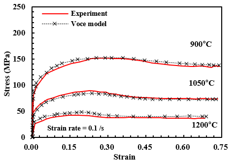
Figure 12.28 Case study of applying the Voce flow stress model to the alloy steel 20MoCrS4 [12.9]
12.5.2.2 Phenomenological Approach
In the previous section, the metallurgical approach was introduced. Although Voce's model is attractive, great difficulty is involved in obtaining the material constants. To resolve this problem, a flow stress model proposed from a phenomenological viewpoint may be realistic. This phenomenological flow stress model includes many material constants, and how to determine these material constants is the pending task.
Many of the phenomenological flow stress models partially utilize Voce's flow stress model. Cingara and McQueen [12.10] formulated the flow stress in the strain-hardening region before the peak stress by the following equation.
This equation was used in the studies of Ebrahimi et al. [12.11], Fereshteh-Sanaiee et al. [12.12], and Meyer et al. [12.9]. The feature of this model equation is that, regardless of the exponent Ch, the flow stress curve passes through the following coordinate and has a slope of 0 at the peak stress. [ (\bar{\varepsilon}_p, \bar{\sigma}_p) ] Therefore, the exponent Ch can be used to pass through the pattern of the flow stress curve, and this exponent is a material constant.
Ebrahimi et al. [12.11] proposed the following flow stress model equation for the purpose of expressing the flow stress in the softening region.
Here, Cs is a material constant. This equation also, regardless of the exponent Cs, has the flow stress curve pass through the coordinate with a slope of 0 at the peak stress, and can be regarded as an improved model of Voce. [ (\bar{\varepsilon}_p, \bar{\sigma}_p) ] Ebrahimi et al. assumed Ch and Cs to be constants, regarded 𝜀̅p, 𝜎̅p, 𝜎̅s, etc., as functions of strain rate and temperature, and proposed a method of graphically determining their values and functional relationships from experimental data. This method has limitations in generalization, and has the problem that extensive experiments must be presupposed to determine the coefficients or functions by the graphical method.
Figure 12.29 shows a case study of a flow stress curve obtained using the Ebrahimi et al. model for the magnesium alloy AZ80 material [12.12].
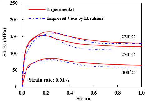
SentenceFigure 12.29 Case study of applying the flow analysis model of Ebrahimi et al. to the magnesium alloy AZ80
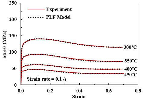
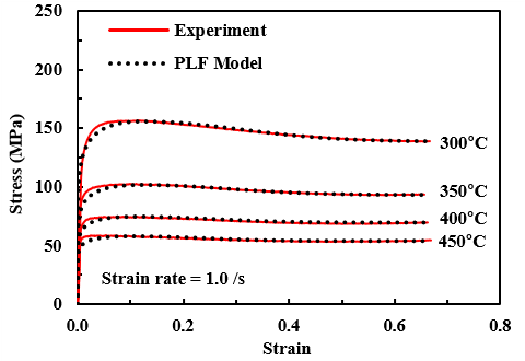
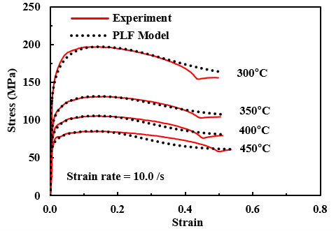
Recently, Kaswandee et al. [12.13], based on the research results of Ebrahimi et al., developed a method that regards all of the following material constants or material properties as functions of strain rate and temperature, and identifies them using an optimization technique. [ C_h, \quad C_s, \quad \bar{\varepsilon}_p, \quad \bar{\sigma}_p, \quad \bar{\sigma}_s ] These material properties are assumed to be piecewise bilinear functions or closed-form functions of strain rate and temperature, and the relevant material constants are determined by a systematic method and optimization technique. Therefore, although there is a disadvantage that many coefficients are defined, to resolve this disadvantage, user intervention in the material constant acquisition process was minimized. Thus, the practical method proposed by Kaswandee et al. simultaneously pursued automation of the coefficient determination process together with the flexibility and accuracy of the results using many material constants and coefficients. Table 12-4 shows the developed mathematical models, and Figure 12.30 shows a case study of applying the PLF model (piecewise bilinear function model) to AHS-2, an alloy steel. Table 12-5 is the information needed to obtain the flow stress curves of Figure 12.30, and was obtained from experimental data.
[Table 12-4] Summary of the PLF model and the CFF model
| Functions | PLF model * | CFF model \(^\S\) |
|---|---|---|
| \(C_h\) | Piecewise bi-linear function | \(C_h = h_1 T + h_2 \dot{\bar{\varepsilon}} + h_3\) |
| \(C_s\) | Piecewise bi-linear function | \(C_s = s_1 T + s_2 \dot{\bar{\varepsilon}} + s_3\) |
| Peak strain, \(\bar{\varepsilon}_p\) | Piecewise bi-linear function | \(\bar{\varepsilon}_p = a_5 + a_1 \dot{\bar{\varepsilon}}^{a_2} e^{a_3 T} + a_4 e^{a_2 / T^m}\) |
| Peak stress, \(\bar{\sigma}_p\) | Piecewise bi-linear function | \(\bar{\sigma}_p = b_5 + b_1 \dot{\bar{\varepsilon}}^{b_2 + b_3 T^m} \bar{\varepsilon}_p^{\,b_4} \left( e^{b_6 / T} + b_8 T \right)\) |
| Steady-state stress, \(\bar{\sigma}_s\) | Piecewise bi-linear function | \(\bar{\sigma}_s = c_5 + c_1 \dot{\bar{\varepsilon}}^{c_2 + c_3 T^m} \bar{\sigma}_p^{\,c_4} \left( e^{c_6 / T} + c_8 T \right)\) |
* PLF (Piecewise bi-Linear Function) denotes formulation using a piecewise linear function.
\(^\S\) CFF (Closed-Form Function) denotes formulation using a function expressed clearly in mathematical form.
[Table 12-5] Information for obtaining the flow stress of AHS-2
| \(\dot{\bar{\varepsilon}}\) (/s) | T (℃) | \(\bar{\varepsilon}_p\) | \(\bar{\sigma}_p\) (MPa) | \(\bar{\sigma}_s\) (MPa) | \(C_h\) | \(C_s\) |
|---|---|---|---|---|---|---|
| 10.0 | 300 | 0.1437 | 196.9100 | 155.8600 | 0.1764 | 3.6964 |
| 350 | 0.1409 | 131.3900 | 104.4800 | 0.1614 | 4.5914 | |
| 400 | 0.1385 | 105.1600 | 78.9700 | 0.1464 | 5.4864 | |
| 450 | 0.1317 | 85.6660 | 61.1940 | 0.1314 | 6.3814 |
⒜0.1/s
⒝1.0/s
⒞ 10.0/s
Figure 12.30 Flow stress curves of the aluminum alloy AHS-2 according to strain rate (case study of applying the PLF model)
12.5.3 Comparison of Flow Analysis Models
Figure 2.31 compares the results of the high-temperature flow stress model formulas for the alloy steel 20MoCr54 material. The experimental flow stress values show typical high-temperature flow stress characteristics of softening after strain hardening, and all flow stress models remain within an acceptable error range. In particular, the PLF model is most similar to the experimental results, followed by the CFF model. The 5-variable Hensel-Spittel model appears to have had some difficulty in expressing softening. The Ebrahimi et al. model is excellent at 1050℃ and 1200℃, but shows a somewhat large difference from the experimental values at 900℃.
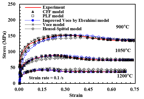
Figure 12.31 Comparison of the results of high-temperature flow stress model formulas for the alloy steel 20MoCr54 material
Figure 2.32 compares the results of flow stress models applied to the magnesium alloy AZ80. In this figure, among the three flow stress curves obtained experimentally, the one at 250℃ differs somewhat from the other two. That is, softening was measured to occur somewhat abruptly. Nevertheless, both the PLF model and the CFF model follow the experimental results well, whereas the Ebrahimi et al. model shows a somewhat large difference from the experimental results. This implies that, since the variables in the PLF model and CFF model are determined by an optimization routine, a natural weighting was applied to the two that are highly similar, whereas in the Ebrahimi et al. model the material constants are determined based on a graphical method, so that, as in this example where one of the three curves differs somewhat from the other two, the variable determination may not be scientific.
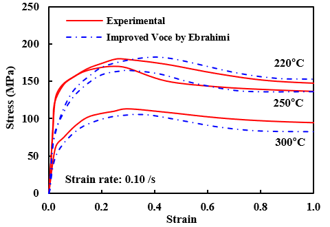
Figure 12.32 Comparison of flow stress models for the magnesium alloy AZ-80
3
12.6 Directionality of Plastic Flow of Metal Materials at Room Temperature
12.6.1 A Study on the Isotropy of Bulk Materials
The method for obtaining flow stress based on the tensile test was explained above. This method has the advantage of providing reliable results even at high strains.
However, in actual forging, although plastic deformation occurs locally in a tensile state, most regions undergo compressive forming. Therefore, the compression test is commonly used for the purpose of measuring the flow stress of a material even at room temperature. Since obtaining the flow stress based on the tensile test was studied in Section 12.4, this section briefly introduces the acquisition of flow stress by the compression test.
The compression test at room temperature is conducted with friction minimized at the contact surface between the die and the material in order to minimize the influence of the barreling phenomenon. The upper limit of strain that can be obtained from a single compression test is around 0.5. Considering that the maximum strain during forging exceeds 2.0, the method relying on the traditional compression test has a clear limitation. However, the compression test has a great advantage in economic terms.
Of course, at room temperature it is theoretically possible to obtain the flow stress at high strain through continuous compression testing, but because somewhat sophisticated experiments are required and there are equipment constraints, this method is generally not widely used. The continuous compression test is a compression test for obtaining the flow stress at high strain by removing the bulged part of the compressed specimen to make a new specimen and continuously testing the strain-hardened specimen.
Recently, a technique for characterizing the flow stress characteristics of a material considering barreling and compression simultaneously using an optimization technique has been used. This method provides the flow stress for relatively high strains. The yield theory studied in Chapter 4 is based on the assumption of isotropy. The assumption of isotropy is somewhat far from the reality of most metal materials. The anisotropy of sheet materials has a large effect on the plastic deformation of metals. Therefore, understanding the isotropy and anisotropy of metal materials can directly or indirectly influence the acquisition of the solution and the evaluation of the results.
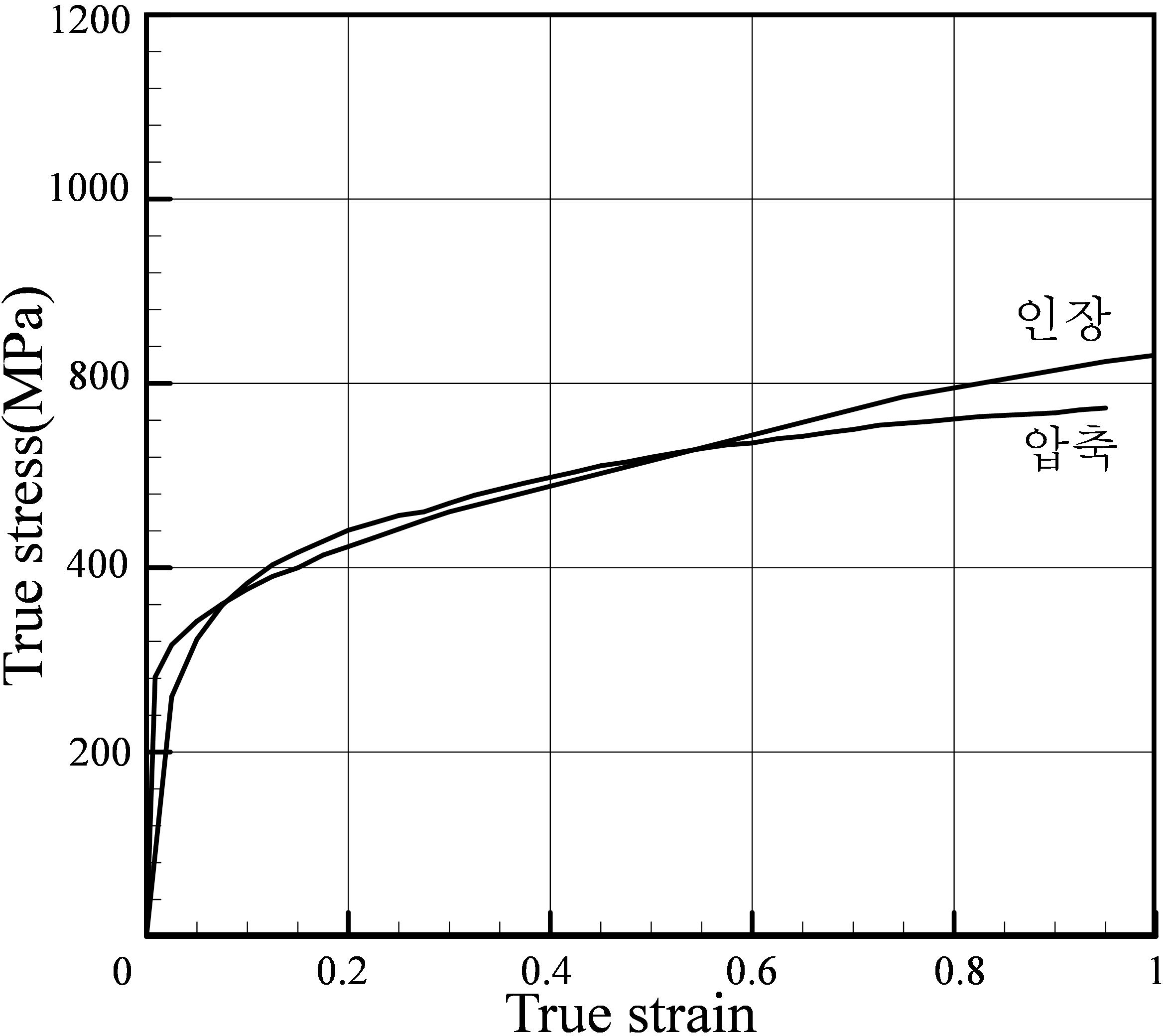
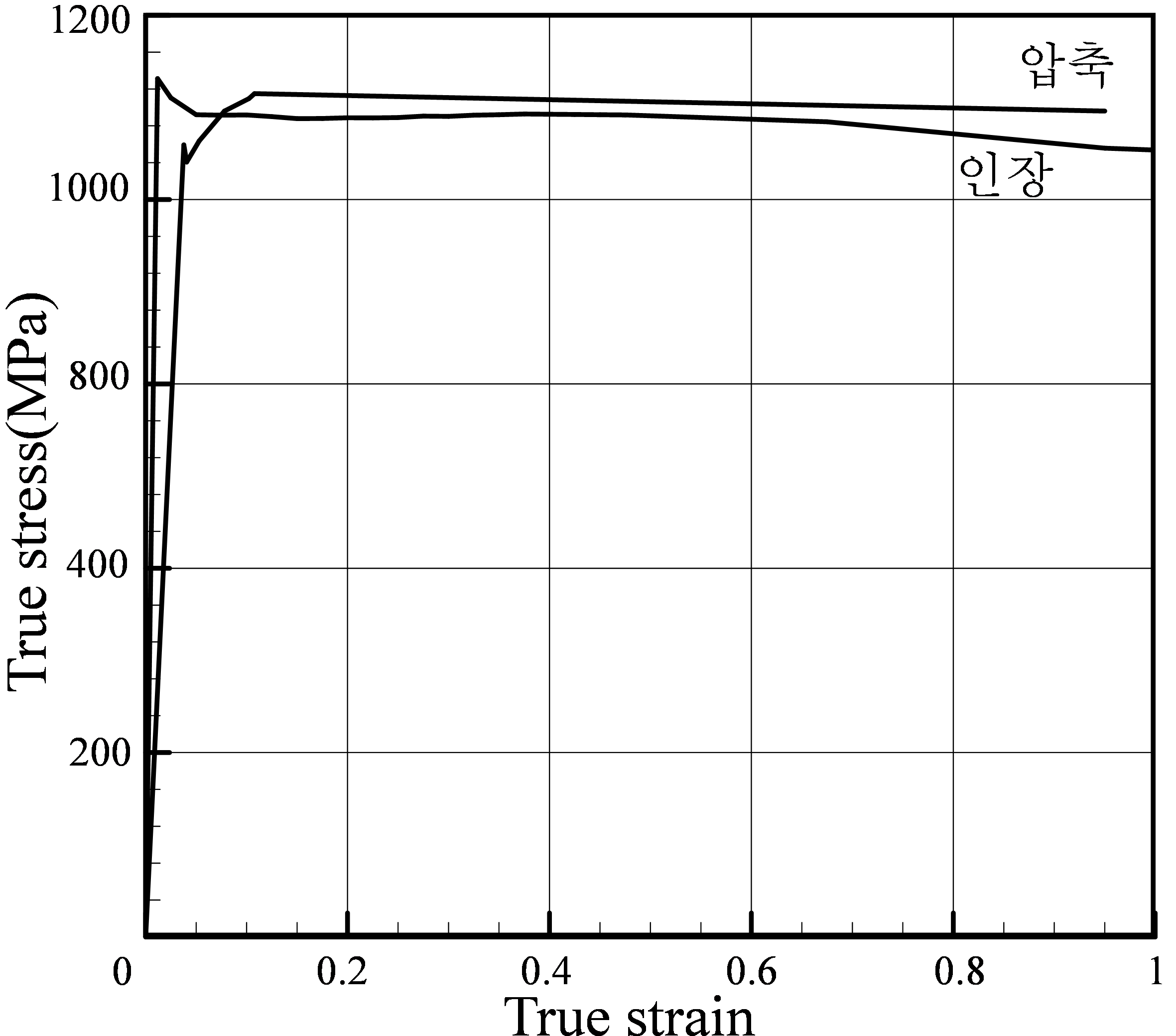
Here, by comparing the flow stress of SCM435 and ESW105 obtained by compression tests and tensile tests, the isotropy of bulk materials pretreated for forging is studied. Figure 12.33⒜ compares the flow stress of SCM435, and Figure 12.33⒝ compares the flow stress of ESW105. In these two results, the flow stress of the materials obtained by the tensile test and the compression test shows a similar tendency.
⒜SCM435
⒝ESW105
Figure 15.5 Design variables and convergence characteristics
In general, since forging undergoes more compressive deformation than tensile deformation, flow stress information obtained by compression testing for a room-temperature material will be more useful than flow stress information obtained by tensile testing. However, there is a problem that the accuracy decreases as the strain increases. In contrast, results obtained using a material-property acquisition technique that uses tensile test results relatively include the flow stress for high strains. Therefore, securing a flow stress curve that appropriately utilizes both results must precede the advancement of metal forming simulation utilization technology. In particular, since the plastic flow characteristics of metal materials at room temperature are highly dependent on pretreatment, the idea that materials with the same manufacturing process and composition have the same characteristics should be discarded.
12.6.2 A Study on the Bauschinger Effect
In general, press forging performs heat treatment such as annealing between stages. This has the effect of reducing strain hardening and, consequently, enhancing the validity of the isotropy assumption.
However, in automatic multi-stage cold forging, which has been continuously developing recently, no special heat treatment process can intervene between stages. In such cases, a material that has undergone compressive deformation may undergo tensile deformation, and vice versa. When a material is plastically deformed by an applied yield stress and then plastically deformed in the opposite direction, the yield stress tends to decrease even though it is a strain-hardening material. A typical example is shown in Figure 12.34. This phenomenon is explained by the Bauschinger effect.
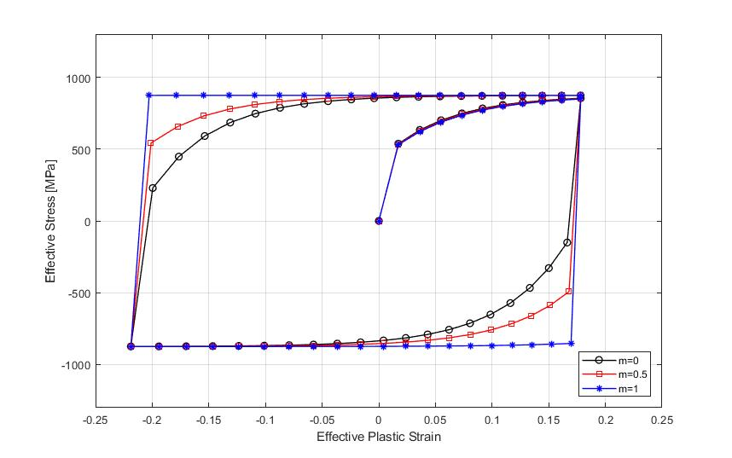
Figure 12.34 Bauschinger effect m=0: nonlinear kinematic hardening model; m=0.5: combined hardening model;
In many cases, drawn wire rod is fed into cold forging. Such cases are especially common in automatic multi-stage cold forging. However, since drawing basically relies on tensile deformation, whereas forging generally relies on compressive deformation, it is relatively strongly influenced by the Bauschinger effect in terms of flow stress. The Bauschinger effect refers to the property in which the stress-strain characteristics of a material change due to the microscopic stress distribution imposed on the material by plastic deformation. Due to this property of the material, plastic deformation by tensile stress results in a decrease in the compressive strength of the material. Of course, the reverse also holds. This phenomenon generally occurs in polycrystalline metal materials.
The Bauschinger effect lowers the strength of the material, so it has many negative aspects. However, in the metal forming of low-strain-hardening high-strength materials, the effect can be utilized for the purpose of minimizing the forming load [12.14]. Although materials with high strain-hardening capacity also have the Bauschinger effect, since the strain hardening due to tensile or compressive deformation is much larger than the Bauschinger effect due to the opposite deformation, the influence on the forming load as described above may not be large.
On the other hand, understanding the compressive flow stress characteristics of a material after a drawing process that relies on tensile deformation has important meaning in terms of the utilization of metal forming simulation technology. In this section, the compression characteristics of drawn SCM435 coil material are experimentally quantified from the viewpoint of the Bauschinger effect. The experiment consists of two stages. The first stage is the drawing process of the base material. Prior to drawing, the coil-shaped base material was coated and lubricated, and base materials were produced under reductions of area of 10%, 20%, 30%, 40%, and 50% through drawing. The specimens for compression testing were fabricated in accordance with the standard ASTM E9. The height of the specimen is 15.0 mm and the diameter is 10.0 mm.
The concerns regarding the drawing process are the distribution of effective strain according to the reduction of area and the distribution of principal stress during deformation. Such information can be obtained relatively accurately by metal forming simulation technology based on the finite element method. Figure 12.35 shows the predicted results of the drawing process obtained using the tensile flow stress of SCM435 presented in Figure 12.33. Since the drawing process is characterized by low friction, 0.03 was used as the friction coefficient. The compression test was conducted in accordance with ASTM E9. Three repeated tests were performed for each test, and as a result, the deviation was negligibly small. Figures 12.36⒜ and 12.36⒝ are the compression test results. Figure 12.36⒜ is the stress-strain curve, which was prepared under the assumption that the initial strain is 0.0. From this figure, the strain hardening due to the drawing process can be confirmed, and it can be confirmed that during the compression test the strain-hardening capacity is lost initially and is recovered again after a certain amount of deformation.
The region in which the strain-hardening capacity is lost appears proportional to the drawing ratio, i.e., the reduction of area. Figure 12.36⒝ is drawn by shifting Figure 12.36⒜ to the right by the estimated initial strain (i.e., the average effective strain of Figure 12.35), for the purpose of quantitatively investigating the Bauschinger effect. From Figure 12.36⒝, it can be seen that, within the investigated range and regardless of the drawing ratio, the yield stress decreases almost constantly due to the Bauschinger effect. And the perfectly plastic characteristic maintained for a certain period after yielding occurs is linearly proportional to the drawing ratio, and the size of that region is 30% of the average effective strain caused by drawing.
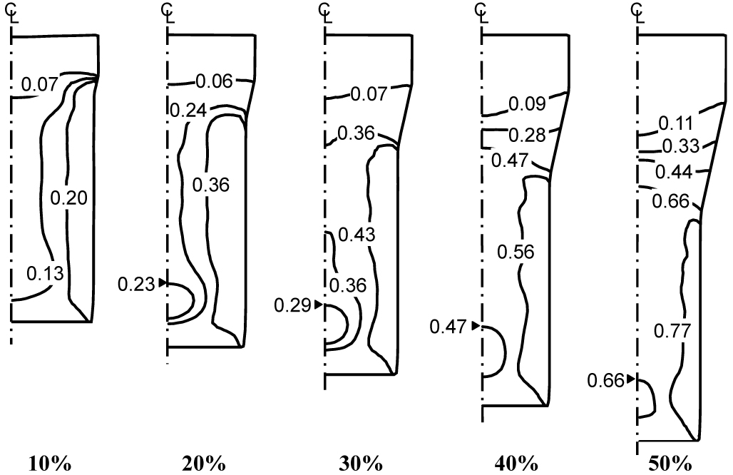
Figure 12.45 Metal flow lines, temperature distribution, and cracks at the final forming instant
As shown in Figure 12.36⒜, in the case of SCM435, the decrease in flow stress due to the Bauschinger effect (Figure 12.36⒝) fundamentally cannot overcome the strain hardening due to tension. In other words, no matter which drawn material is used, the compressive load under the same conditions increases because of strain hardening. And it can be seen that when compressive deformation is applied to a material that has undergone strain hardening due to tensile deformation, the form of the flow stress is greatly influenced by the degree of tensile deformation. This has great implications from the viewpoint of most plasticity theory and applications based on the assumption of isotropy. From Figure 12.36⒝, in the case of SCM435, from the viewpoint of the currently accumulated effective strain, the compressive flow stress of the drawn material appears somewhat smaller than the compressive flow stress of an initially undeformed specimen that has undergone the same compressive deformation, due to the Bauschinger effect, and it tends to show perfectly plastic characteristics over a certain region immediately after initial yielding.
On the other hand, the flow stress characteristics of a material for which strain hardening can be neglected, such as ESW105, tend to be exactly the opposite of those of the aforementioned SCM435. For example, if a drawn ESW105 specimen is compression-tested, it shows the property of strain hardening within a certain range, and the compressive load tends to decrease due to the Bauschinger effect. The detailed description of this is replaced by the reference [12.14].
In conclusion, the plastic flow characteristics of a material at room temperature, i.e., the strain-hardening capacity and the magnitude of the flow stress, are highly dependent on the manufacturing process and heat treatment process. Therefore, deep understanding of the material together with continuous test evaluation is required.
The following example eloquently demonstrates the importance of the foregoing. The analysis results of the heading process presented in Figure 12.37 emphasize the influence of strain-hardening capacity on cold forging. As a result of applying the conditions of Figure 12.37⒜, i.e., the initial flow lines and effective strain, identically to SCM435 (a strain-hardening material) and ESW105 (a material for which strain can be neglected), the plastic flow appears greatly different. This process applies the ESW105 material to a process developed for SCM435. Therefore, from the viewpoint of filling the die cavity by the material, it is natural that SCM435 looks good. If one had started from initial process shape information suitable for ESW105, the result would be the opposite. It is emphasized that this example is to emphasize that the characteristics of the two materials differ from each other, not to reveal the superiority of any material.
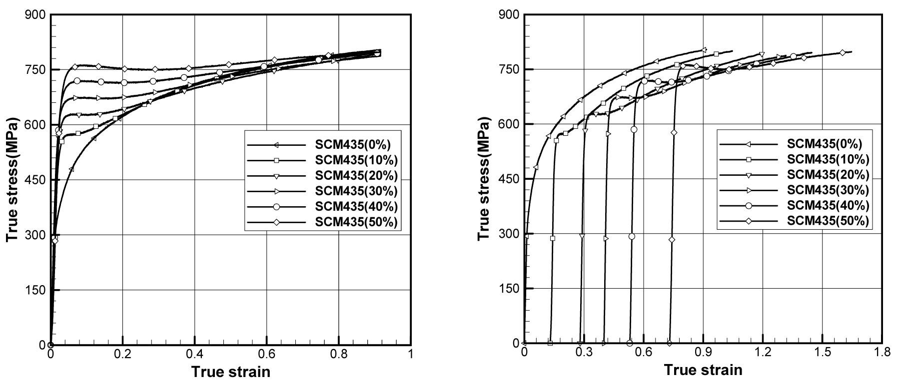
Figure 12.36 True stress–true strain curves obtained by compression testing
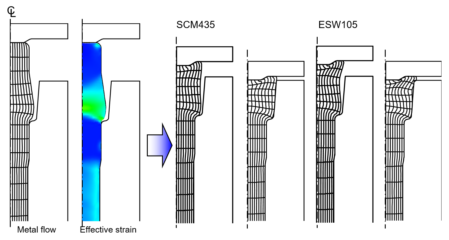
Figure 12.37 Influence of strain-hardening capacity on plastic deformation
12.7 Fracture of Materials During Metal Forming
12.7.1 Ductile Fracture Case – Central Bursting
Extruded shaft-type products are used as key components for power transmission, etc., but an automobile using a product in which central fracture has occurred can lead to an unexpected major accident. Therefore, the central fracture problem that can occur during extrusion is both a design consideration regarded as important in industrial fields and a subject of quality control. Central fracture also occurs in drawing or wire drawing, and this phenomenon is a cause of many problems not only during the process but also during use.
Summarizing existing studies, in addition to the macroscopic and microscopic state of the material, process design variables, i.e., the friction coefficient, the extrusion and drawing die angles, the reduction of area, etc., influence the occurrence of central fracture, and there exists an optimal design from the viewpoint of central fracture.
According to ductile fracture theory, fracture of a material during plastic deformation occurs when the accumulated damage value reaches the damage tolerance limit, i.e., the critical damage. Therefore, in ductile fracture theory the fracture phenomenon is determined by the critical damage and the accumulated damage. The critical damage is a property of the material and, empirically, is relatively strongly influenced by the composition of the material, the degree of inclusion of impurities, and heat treatment.
To generate cracks, an appropriate numerical technique is needed. Representative techniques include the element deletion technique, the element degeneration technique, the element boundary separation technique, and the crack propagation technique. From the standpoint of programming the numerical technique, the crack propagation technique is the most difficult, but its accuracy is relatively high. However, the crack propagation technique is not realistic for 3D application due to the complexity of the mesh. The element deletion technique is simple, but has some problems. For example, it is not easy to solve the problem that occurs when the fracture surfaces contact each other and friction occurs after a crack has formed. To resolve such problems, the element deletion technique combined with the element degeneration technique can be effective.
In this section, the central fracture phenomena occurring in the multi-stage drawing process and the extrusion process are analyzed, and their results are compared and examined to promote understanding of the central fracture phenomenon.
Damage causes softening of the material. Therefore, damage influences the flow stress, so the flow stress is a function of damage. Attempts have been made to link the relationship between damage and flow stress to reflect the influence of damage, but since the influence of damage is not large, from an engineering standpoint the damage can be regarded as constant in the current analysis step and its influence can be reflected. In this case, multiplying the existing flow stress function by a function reflecting the influence of damage can be a realistic alternative. For example, the following flow stress function can be an example.
Here, \(\delta(D)\) has a value less than or equal to 1. \(D\) is the damage. In continuum damage mechanics, damage is defined as follows.
The flow stress mathematical model requires the input of material constants by the user. The material constants are obtained by material testing and curve fitting using a mathematical model. The information obtained through material testing is obtained by curve fitting methods based on the least-squares method, etc.
12.7.1.1 Extrusion Process
Figure 12.38 shows the predicted results of a central fracture occurring during the extrusion process, predicted using the element boundary separation technique for visualization. In this example, the flow stress of the SWCH10A material (see graph 5 of Figure 12.18) was used for the compression process analysis, and the critical damage value was set low to forcibly induce central fracture. Therefore, it is unrelated to actual central fracture. However, the results can help in understanding the central fracture phenomenon and the approach method.
Figure 12.38 shows the influence of the extrusion angle on the chevron crack when the reduction of area is 25% and the friction coefficient is 0.03. The normalized Cockcroft-Latham damage model was used for the purpose of element boundary separation.
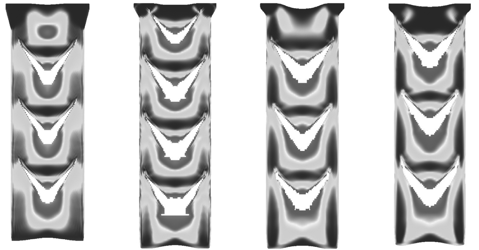
Figure 12.38 The conditions of the influence of the die angle on central fracture (R.A. = 25%, \(\mu = 0.03\)) are as follows.
According to a literature survey [12.15], the experimental value of the normalized maximum central fracture diameter, defined as the maximum diameter of central fracture divided by the material diameter after extrusion, is around 0.85. And the shape of the central fracture is a V-shape with a sharp tip. That is, the central fracture occurring in the extrusion process is called a crack in the shape of a flying bird, i.e., a chevron crack. Therefore, the predicted results of the central fracture that can occur in the extrusion process of Figure 12.38 qualitatively agree with the experimental results presented in the literature.
12.7.1.2 Drawing Process
Table 12-6 summarizes the process design of a hypothetical 6-stage drawing process, i.e., the radius at each stage. The initial radius and length of the material used in the multi-stage drawing process are 7 mm and 21 mm, respectively, and 3675 quadrilateral elements with a side length of 0.2 mm were used as the initial mesh. A conical die was used, the die angle was assumed to be \(\alpha = 10^{\circ}\), and the friction coefficient was assumed to be \(\mu\) = 0.02. The die land was set to 1.5 mm, and the corner radius was set to 2.0 mm. The material is SWCH10A, and as initial conditions the strain and damage were regarded as zero.
[Table 12-6] Radius of the material in the 6-stage drawing process
| Stage | 1 | 2 | 3 | 4 | 5 | 6 |
|---|---|---|---|---|---|---|
| Entrance | 7.0 | 6.65 | 6.3 | 6.0 | 5.7 | 5.4 |
| Exit | 6.65 | 6.3 | 6.0 | 5.7 | 5.4 | 5.15 |
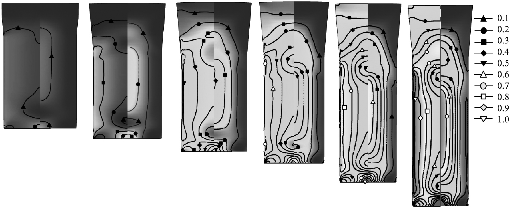
Figure 12.39 Analysis of the multi-stage drawing process without considering central fracture – effective strain (left) and damage (right)
The element boundary separation technique and the normalized Cockcroft-Latham damage model were used for the purpose of predicting cracks. Figure 12.39 shows the analysis results of the 6-stage drawing process obtained without considering central fracture. The left side is the effective strain, and the right side is the damage. As an analysis result, the maximum damage at the end of stage 5 is 0.67. Therefore, to induce central fracture at stage 6, the critical damage was assumed to be 0.71 to predict the central fracture phenomenon. To prevent softening of the state variables due to mesh reconstruction during analysis, mesh reconstruction was not performed.
From the predicted results of central fracture in Figure 12.40, it can be seen that, unlike the extrusion of Figure 12.38, the shape of the central fracture is a U-shaped cup with a convex tip. The normalized maximum diameter of the central fracture was 0.36, and the normalized height was 0.22. These values differ greatly from those of a typical extrusion process.
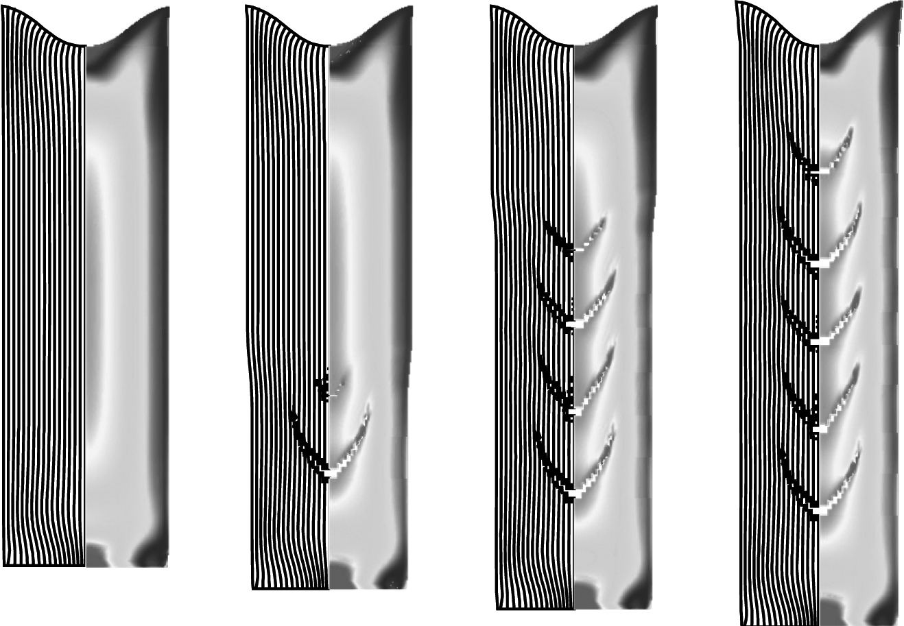
Figure 12.40 Prediction of central fracture occurring in the multi-stage drawing process – damage distribution
The main cause of the aforementioned difference can be found in the geometric characteristics of the process. As shown in Figure 12.41, the reduction of area of the extrusion process in which central fracture occurs is relatively large compared to each drawing process, and for this reason confined extrusion is common. And the angle of the conical die is relatively large.
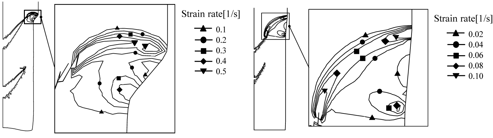
Figure 12.41 Central fracture and shear band of the extrusion process and the 6-stage drawing process
12.7.2 Hot Brittle Fracture Case
Figure 12.42 shows the automatic multi-stage hot forging process diagram used in the hot brittle fracture analysis, together with the plastic flow lines obtained as predicted results.
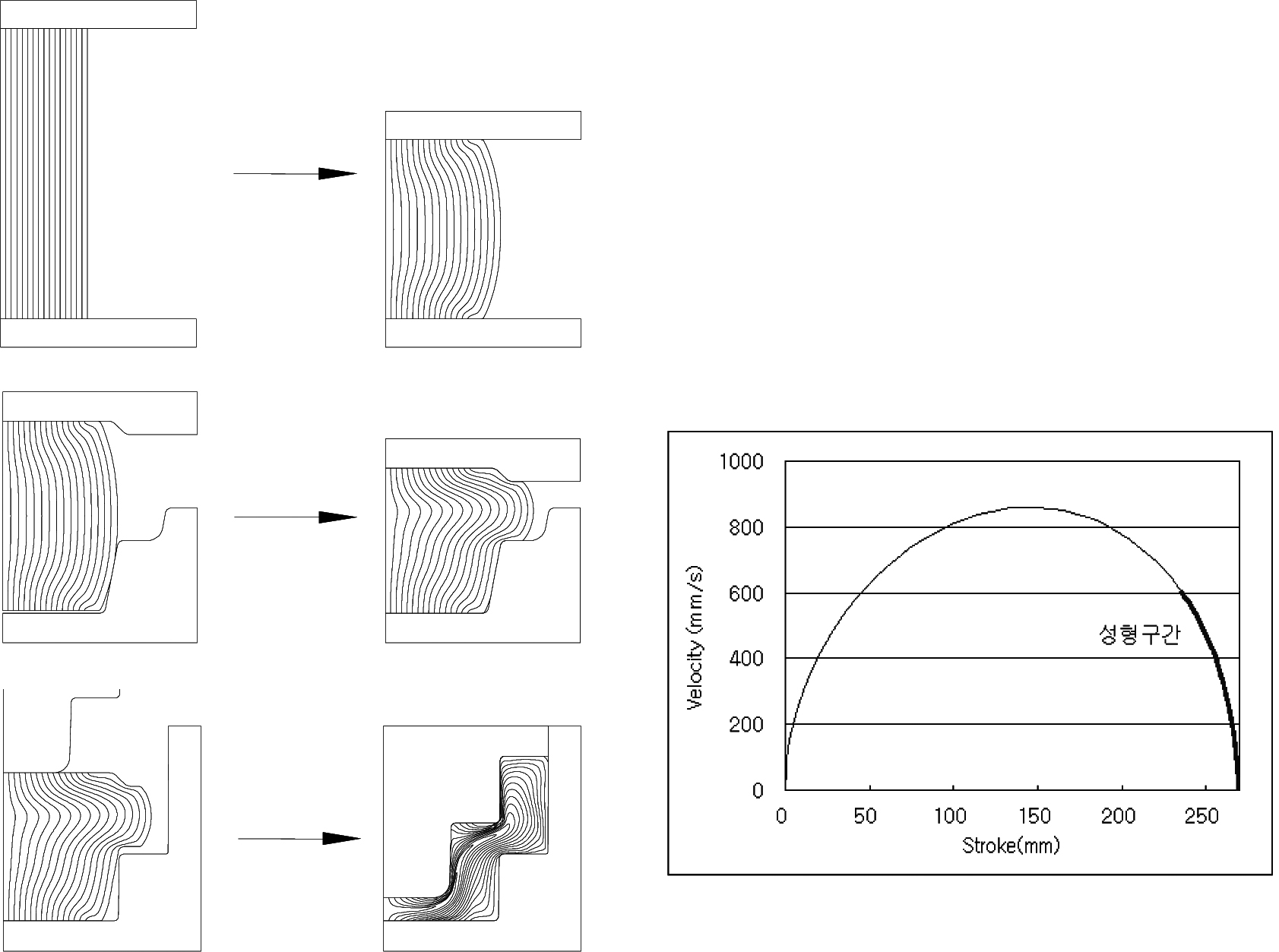
The process conditions and variables determined based on references and experience are as follows [12.2]. Initial material temperature: 1150℃; initial die temperature: 150℃; die speed: slider-crank press; rotation speed: 60 rpm; total stroke: 270 mm; ram length: 810 mm; flow stress: Table 4-4; Coulomb friction coefficient: \(\mu = 0.3\); convective heat transfer coefficient: \(h_c = 2.95 \text{ W/mm}^2\text{°C}\) ; heat transfer coefficient between material and die: \(h_i = 30.0 \text{ kW/mm}^2\text{°C}\) .
To predict the temperature distribution of the material during the hot forging process, rigid-thermoviscoplastic finite element analysis was performed. Figure 12.44⒜ is the coupled analysis result, showing the temperature distribution of the material immediately after the final forming process in the hot forging process. Figure 12.44⒝ shows the strain rate distribution of the material immediately before the final forming process.
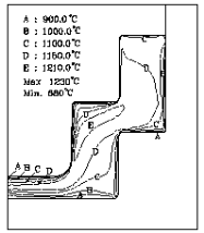
(a)
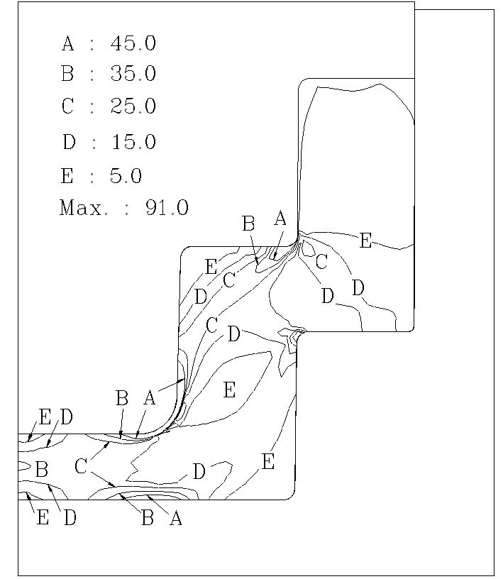
(b)
Figure 12.44 Analysis results at the end of forming ⒜ and immediately before the end ⒝
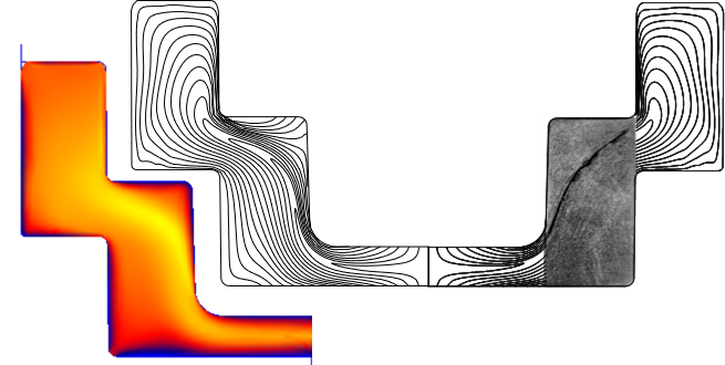
Figure 12.45 Metal flow lines, temperature distribution, and cracks at the final forming instant
As shown in Figure 12.45 (right), the metal flow lines are severely distorted in a specific part. This is because the material underwent severe local deformation during the hot forging process. As shown in Figure 12.44⒜, the maximum temperature appeared in the part where severe local deformation of the material occurred.
As a result of the coupled analysis, the material temperature immediately before forming decreased by about 10℃ due to natural air cooling. The material temperature after forming dropped sharply to 680℃ at the die contact region, while inside the material it rose to a maximum of 1230℃ due to plastic heat. The reason that the temperature drop is relatively small in some of the regions where die contact occurred is that the plastic heat and friction heat due to extreme plastic deformation in the surroundings were relatively large. As a result of the analysis, during the hot forging process the STB2 bearing steel undergoes severe local deformation in the region around contour E in Figure 12.44⒜, and as a result, the temperature rose by up to 80℃ above the initial heating temperature. This temperature rise is judged to be the cause of the internal and external cracks in the material, as shown in Figure 12.45. This is because STB2 exhibits the property of hot brittleness in which the elongation drops sharply at 1200℃. For details on this, please refer to Section 12.2.
12.7.3 Shearing, Piercing, Trimming, and Fine Blanking Processes
The processes that utilize fracture during the process are the shearing, piercing, trimming, and fine blanking processes. Since a fracture prediction case for an axisymmetric process was already introduced in Section 12.7.2, this section introduces cases of 3D application of fracture phenomenon prediction technology.
In 3D problems, because the connectivity information between finite elements is complex, the application of the element boundary division technique is not easy. The element deletion technique is disadvantageous in terms of generality because of the complex geometric problems that arise after separation. Therefore, cases of applying the element deletion technique combined with the element degeneration technique are shown in Figures 12.46–12.48. Appropriate ductile fracture theory and material constants were used to obtain these results.
As shown in Figure 12.48, the analysis results of the cold shearing process agree well with the experimental results.
The analysis cases of the cold piercing process and the cold trimming process are shown in Figures 12.47⒜ and ⒝, and the analysis case of the fine blanking process is shown in Figure 12.48.
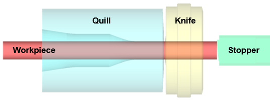
⒜ Initial state of the shearing process
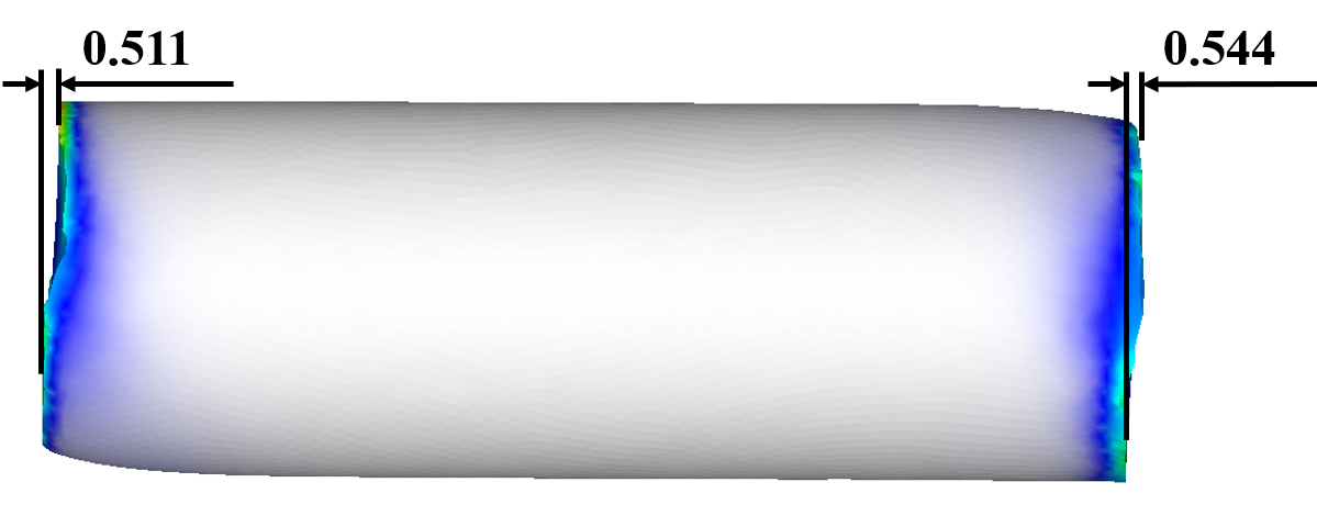
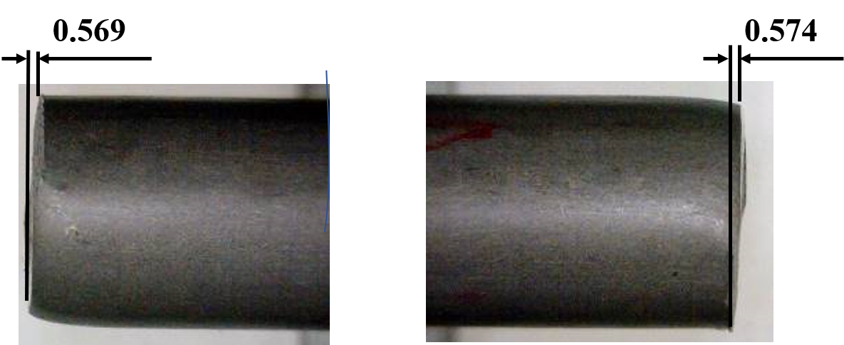
⒝ Prediction (left) and experiment (right) of the shearing process
Figure 12.46 Analysis of the cold shearing process
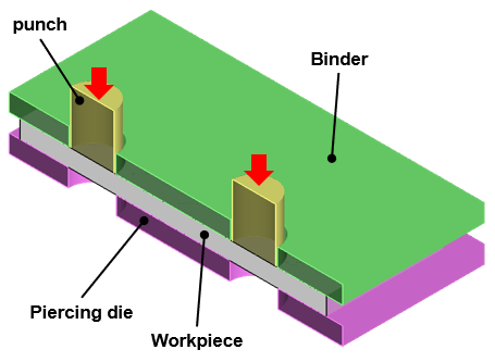
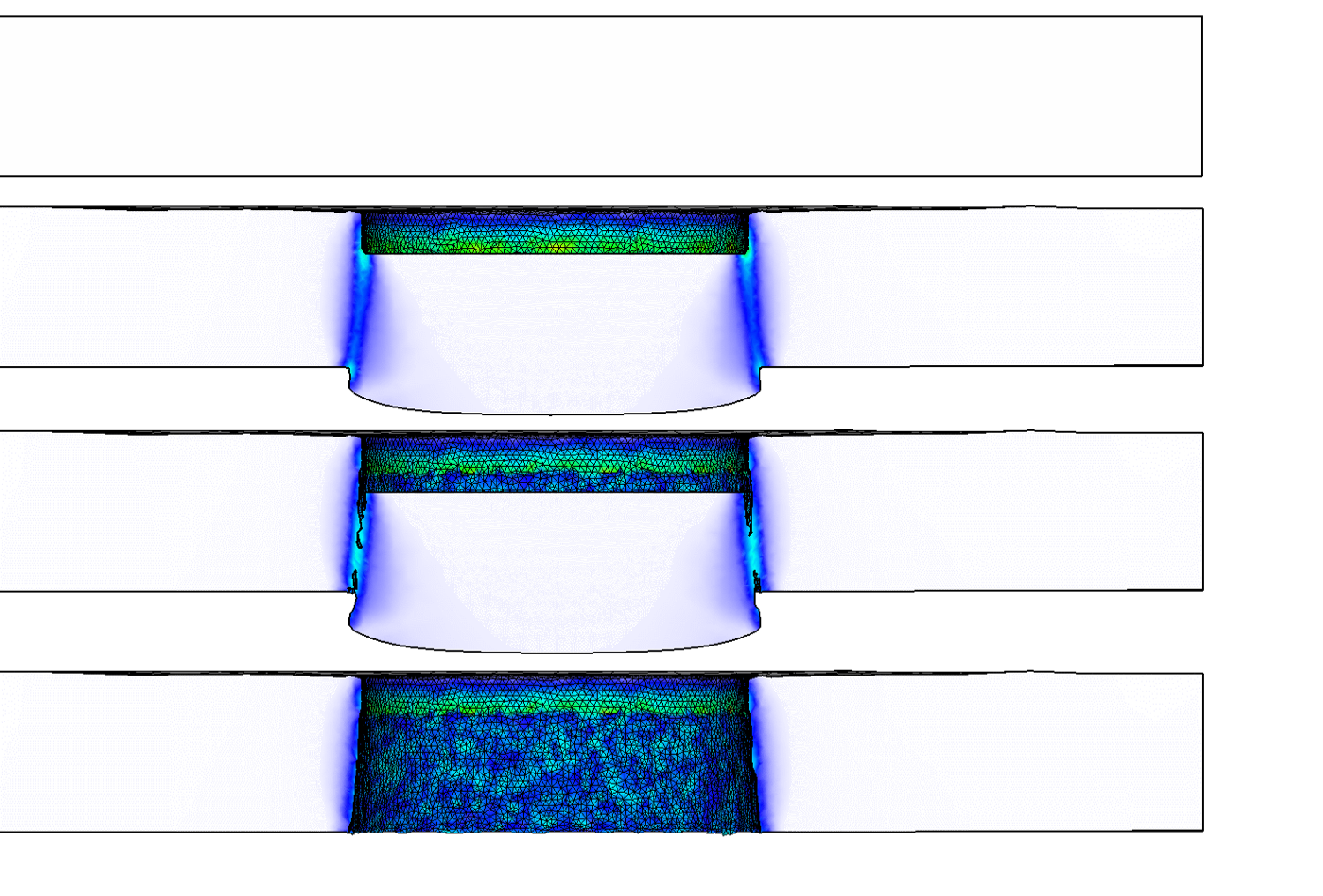
⒜ Cold piercing
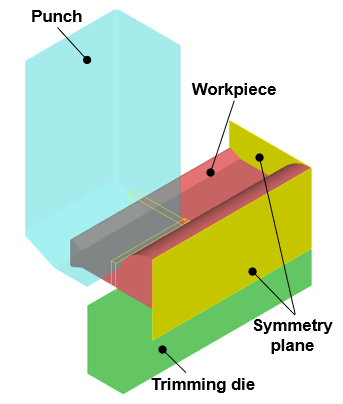
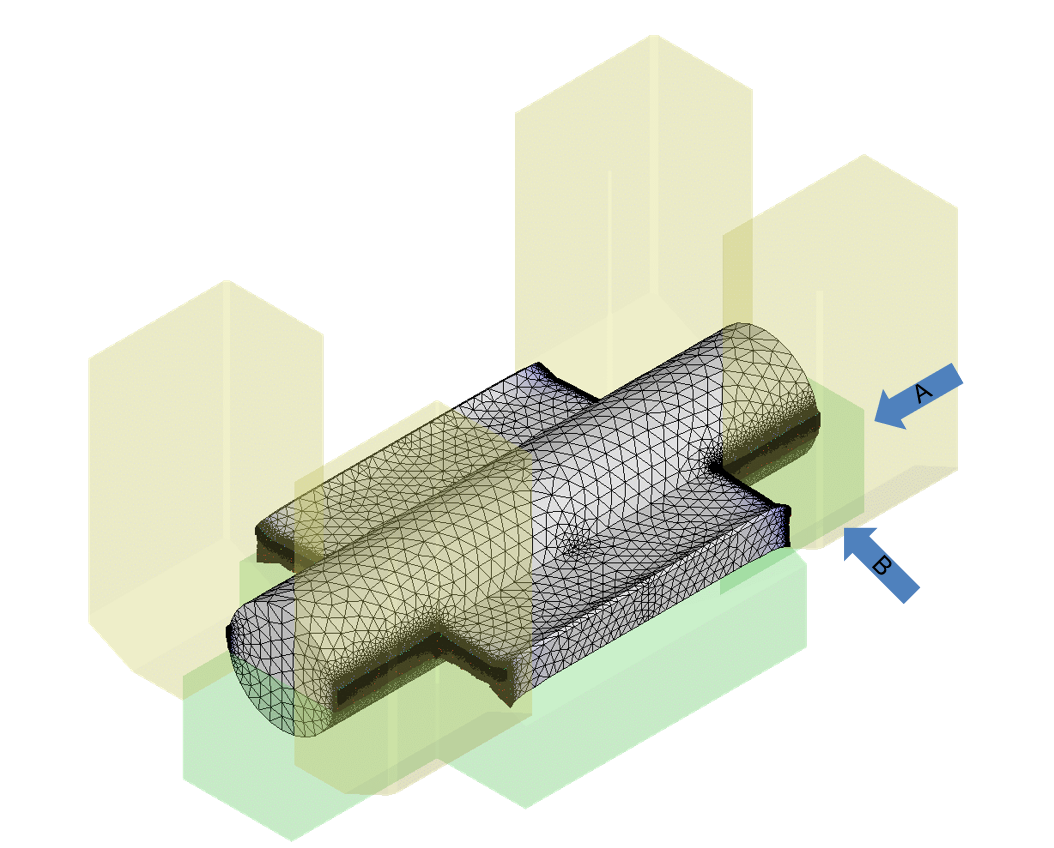
⒝ Cold trimming
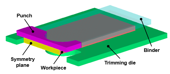
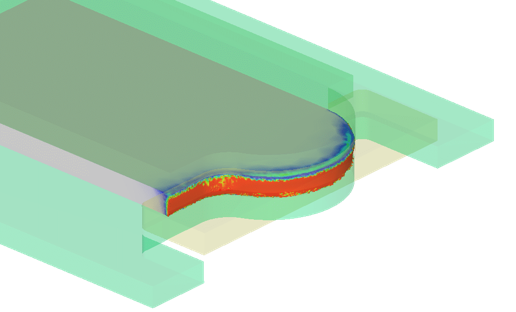
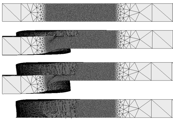
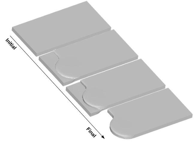
Figure 12.48 Analysis of the fine blanking process