5 Boundary Conditions and Friction

5.1 Boundary conditions

If the governing equation is a differential equation, boundary conditions or initial conditions are essential in order to obtain a unique solution. Boundary conditions are divided into two types. If the governing equation is a differential equation of order \(2p\), a boundary condition involving derivative terms from order \(0\) up to order \(p-1\) is called an essential boundary condition, and a boundary condition involving derivatives from order \(p\) up to order \(2p-1\) is called a natural boundary condition. The boundary conditions of an ordinary differential equation are given as real values at points, and for a partial differential equation they are given as functions whose domain is the boundary.

In elasticity problems, the essential boundary conditions are geometric conditions related to displacement (including angle), and the natural boundary conditions are mechanical boundary conditions related to force (including moment). In plasticity problems, the essential boundary conditions are geometric conditions related to velocity, and the natural boundary conditions are mechanical boundary conditions related to force. In heat-transfer problems, a boundary where the temperature is prescribed is an essential boundary condition, and a boundary where the heat-transfer rate is prescribed is a natural boundary condition.

At a single boundary point, (number of unknowns \(\times p\)) boundary conditions are imposed. For example, in a problem of finding the temperature distribution, the number of unknowns at a single point or coordinate is one, whether in one-dimensional space, two-dimensional space, or three-dimensional space. Therefore, regardless of the geometric dimension, one boundary condition is imposed at one point. However, this is not the case in mechanics problems where displacement or velocity is formulated as the unknown function of a second-order differential equation. At a single point in a two-dimensional plane, two displacement or velocity components are unknowns, and at a single point in three-dimensional space, three displacement or velocity components are unknowns. Therefore, in this class of problems, as many boundary conditions as the number of dimensions must be imposed at a single point.

Meanwhile, in the analysis of metal forming processes, friction is one of the main factors that determine the characteristics of the process. In the rolling process, an appropriate friction stress between the roll and the material is essential. However, excessive friction stress increases the rolling load and accelerates roll wear, so it must be appropriately controlled. In the forging process, friction plays a role in determining the pattern of metal flow, but it reduces the wear life of the die, so it must be appropriately controlled. In cold working, because the deformation resistance is large, the use of lubricants is common practice. In hot working as well, lubricants are frequently used in order to reduce severe die wear. The main factors affecting friction include the contact-surface pressure, the lubrication condition, the relative velocity, the temperature, the material properties, the surface roughness, etc. In metal forming, since the friction surface is under the extreme conditions of high temperature and high pressure, it is not easy to accurately analyze the influence of the friction factors on the friction stress, and this is one of the main concerns of physics, materials science, plasticity, etc.

5.2 Traditional friction conditions

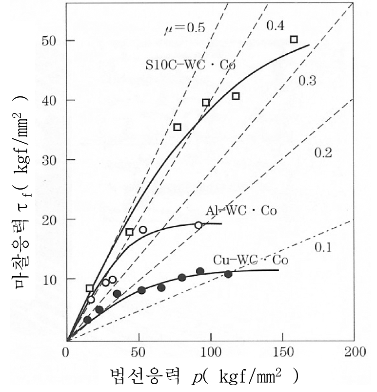
The friction stress is defined by its magnitude and direction. Friction acts in the direction that impedes the motion of the two bodies. The magnitude of the friction stress is a function of the normal stress acting on the contact surface when the two contact surfaces move relative to each other. As shown in Figure 5.1, it is generally known that below a certain value of the normal stress the friction stress is proportional to the normal stress, and above that certain value the dependence of the friction stress on the normal stress decreases. Of course, when the normal stress becomes large, an essentially adhesive state is reached or plastic deformation occurs due to the friction stress, so discussing the magnitude of friction under a large normal stress is somewhat controversial.

Figure 5.1 Normal stress and friction stress [5.1]

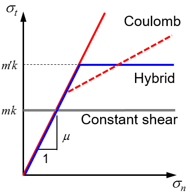
Friction is certainly complex, being a function of the pressure acting on the contact surface, the relative velocity, the temperature, the roughness of the friction surface, the material properties, etc. In plasticity, the friction stress has traditionally been formulated by the law of Coulomb friction and the law of constant shear friction. Recently, the law of hybrid friction, which complements these two friction laws, has also been applied. As shown in Figure 5.2, the Coulomb friction model regards the friction stress as being proportional to the normal stress if relative motion occurs at the contact surface, whereas the law of constant shear friction regards a shear stress equal to a constant fraction of the shear yield stress as acting. If no slip occurs at the friction surface, the shear stress actually acting on the contact surface is smaller than the calculated shear stress (the product of the normal stress and the friction coefficient in the law of Coulomb friction, and the product of the shear yield stress and the friction constant in the law of constant shear friction).

Meanwhile, in the law of constant shear friction, the friction stress is determined independently of the normal stress. It is clear that, since the friction stress is related to the normal stress, the law of Coulomb friction or the friction laws derived from it will reflect actual phenomena better than the law of constant shear friction. However, the law of constant shear friction is widely used for reasons such as its theoretical simplicity and numerical stability. In the friction-sensitive room-temperature ring compression test, it is certain that these two laws predict similar results. However, before using this to justify the law of constant shear friction, one must recall that in ring compression the difference in the stress distribution over the friction surface is relatively small compared with general forging. In extrusion and drawing processes as well, since the variation of the normal stress is relatively small, the two friction laws predict similar results. However, in hot rolling and in geometrically complex hot forging, the exact opposite phenomenon occurs. The details of this are addressed in Section 5.7.

Figure 5.2 Main friction laws

The law of Coulomb friction and the law of constant shear friction are formulated as follows.

(a) Law of Coulomb friction

\[ \sigma_t = -\mu \sigma_n g(v_t - \bar{v}_t) \tag{5.1} \]

(b) Law of constant shear friction

\[ \sigma_t = mk g(v_t - \bar{v}_t) \tag{5.2} \]

Here, \(\mu\), \(m\), \(k\) are the friction coefficient, the friction constant, and the shear yield stress (\(k = Y/\sqrt{3}\)), respectively. \(g(v_t - \bar{v}_t)\) is a function that reflects the influence of the relative velocity \(v_t - \bar{v}_t\) on the friction stress. That is,

\[ g(v_t - \bar{v}_t) = \begin{cases} -1 & \text{if} \quad v_t > \bar{v}_t \\ 1 & \text{if} \quad v_t < \bar{v}_t \end{cases} \tag{5.3} \]

If no slip occurs between the die and the material, the following condition must be imposed on the law of Coulomb friction.

\[ |\sigma_t| \le k \quad \text{if} \quad v_t = \bar{v}_t \tag{5.4} \]

The following function, i.e. the friction-smoothing function, is widely used as a function that satisfies these two conditions while simultaneously accounting for the numerical difficulties that arise when \(|v_t - \bar{v}_t|\) is very small.

\[ g(v_t - \bar{v}_t) = -\frac{2}{\pi} \tan^{-1} \left( \frac{v_t - \bar{v}_t}{a} \right) \tag{5.5} \]

Here, \(a\) is a very small positive real number compared with \(|\bar{v}_t|\), and making \(a\) extremely small brings Eq. (5.5) close to Eq. (5.3).

The point to be emphasized here is the fact that if a converged solution satisfying the yield condition has been obtained using Eq. (5.5), then even in the law of Coulomb friction the friction stress does not exceed the value \(k\). If \(|\mu\sigma_n|\) exceeds \(k\), then \(|v_t - \bar{v}_t|\) of the converged solution becomes sufficiently small so as to satisfy the condition of Eq. (5.4). Ultimately, an adhesion condition is produced. If a converged solution has been obtained rigorously using Eq. (5.5), then even when the law of Coulomb friction is used, the condition of Eq. (5.4) is automatically satisfied.

5.3 Hybrid friction law

Although the friction phenomenon involves some uncertainty, it is generally known that the Coulomb friction law is effective at low contact pressure. Although there is an argument that, because the Coulomb friction law is problematic at high contact pressure, the law of constant shear friction is preferable at high contact pressure, in two dimensions the problem is in fact not an issue because the friction-smoothing function used together with the friction law in the finite element method naturally resolves the problem that the Coulomb friction law poses at high contact pressure [5.2]. However, in three-dimensional problems, there is a disadvantage in terms of computation time in obtaining a sufficiently converged solution that accounts for the friction-smoothing function under high pressure. To resolve this problem, as shown in Figure 5.2, the hybrid friction law can be effective, in which the Coulomb friction law is used at a constant pressure and the law of constant shear friction is used when a pressure greater than that acts, but using an appropriate friction constant (hereafter referred to as the limit frictional factor), i.e. a value somewhat larger than the traditional friction constant used when the whole is regarded as governed by the law of constant shear friction. If the limit frictional factor used in the hybrid friction law is set equal to the traditional friction constant, then the hybrid friction law yields a result that predicts a smaller friction stress at low pressure compared with the conventional law of constant shear friction. If the purpose of the hybrid friction law is to reflect the nonlinearity that occurs at high pressure, then the use of a limit frictional factor somewhat larger than the traditional friction constant is recommended. The hybrid friction law is formulated as follows.

\[ \sigma_t = \begin{cases} -\mu\sigma_n g(v_t - \bar{v}_t) & \text{if} \quad -\mu\sigma_n \le m'k \\ m'k g(v_t - \bar{v}_t) & \text{if} \quad -\mu\sigma_n > m'k \end{cases} \tag{5.6} \]

Here, \(m'\) is the limit frictional factor. The friction stress is a function of the normal stress. In drawing and open extrusion processes, since the variation of the normal stress is relatively small over the entire contact region of the die, the law of constant shear friction and the law of Coulomb friction yield similar results. However, in the rolling process and in forging processes with relatively complex deformation patterns, the use of the law of constant shear friction may be inappropriate for the purpose of plastic flow analysis. The hybrid friction law can help resolve this problem.

5.4 State-variable dependence of the friction coefficient and friction constant

In general, both the friction coefficient and the friction constant are, in most cases, treated as constants. However, since the lubricant film of a lubricated material is broken down during plastic deformation, these values change. They are also affected by temperature and pressure. There are problems in which such changes must be taken into account. Therefore, in order to reflect such phenomena, the friction coefficient and the friction constant may be regarded as functions of temperature, pressure, and the strain of the material as follows.

\[ \mu = \mu_0 W_T(T) W_P(P) W_E(\bar{\varepsilon}) \tag{5.7} \]

\[ m = m_0 W_T(T) W_P(P) W_E(\bar{\varepsilon}) \tag{5.8} \]

Here, the functions \(W_T(T)\), \(W_P(P)\), \(W_E(\bar{\varepsilon})\) can be formulated as various functions, including piecewise-linear functions.

Let us call the use of such a friction coefficient and friction constant a weighted frictional model. That is, the weighted Coulomb friction law refers to the case where Eq. (5.7) is used for the definition of the friction coefficient.

Determining the state-variable dependence of the friction coefficient and friction constant is not easy. However, when regions with severe lubricant-film damage during metal forming are dominant to some extent, this functional relationship must be utilized.

For example, the shape of the aluminum hot-forged product in Figure 5.3(a) cannot be predicted with a constant value of the friction constant or friction coefficient. Figure 5.3(b) shows the results analyzed by the rigid-thermoviscoplastic finite element method using a constant value of the friction constant or friction coefficient, in which the side shape of the observed object differs greatly from one another.

For the forming of this product, a lubricant coating is formed on the material. This lubricant coating faithfully performs its lubricating role until a certain condition is reached, and upon reaching a critical value, it loses its lubricating performance or its performance drops markedly. Regarding the factor that governs the performance of this lubricant coating as lying in the strain of the material at the contact surface, and treating the friction coefficient as increasing greatly upon reaching a critical surface strain, the analysis yielded results similar to the experiment, as shown in Figure 5.3(c). It was visually confirmed that in the contact region where the actual strain exceeded the critical surface strain, the lubricant film was severely damaged and the material and die came into direct contact. On the other hand, as shown in Figure 5.3(a), on the side surface of the observed object the lubricant film remained good enough to be visually confirmed even after the completion of forming.

(a) Experiment

(b) Constant friction coefficient or friction constant

(c) Strain-dependent friction coefficient or friction constant

Figure 5.3 Aluminum piston hot forging case

5.5 Wear

The wear phenomenon is affected by the material properties, state variables, surface roughness, lubrication, etc. The main factors are the frictional dissipation energy, the material properties and temperature at the contact surface, the surface roughness, the lubrication condition, etc. The frictional dissipation energy is a function of the friction stress and the sliding distance (i.e. the relative displacement at the contact surface). Among the material properties, hardness is representative, and hardness has a temperature-sensitive nature. Surface roughness and lubrication condition have a direct influence on the friction coefficient or friction constant and therefore greatly affect wear. Failures due to wear can be broadly classified into surface fatigue failure, abrasive failure (or grinding wear), adhesive failure, corrosive failure, etc. The wear phenomena that occur in metal forming are explained broadly by two types, i.e. abrasive wear and adhesive wear.

The abrasive wear phenomenon is caused by the friction surface being ground by abrasives, high-hardness impurities, or protrusions of a hard surface present on the two friction surfaces coming into contact with a soft surface. Therefore, one of them is severely worn away, and the material properties of the counterpart material have a great influence on wear.

Adhesive wear is the wear that occurs by the phenomenon in which parts of the two materials fuse together and then break away. That is, the phenomenon in which the micro-protrusions of the two bodies brought into contact by the mechanical interlocking of the contact surface adhere under high pressure through the physical phenomena of diffusion and melting, and are then separated by relative motion, is called adhesive wear. Adhesive wear is a mechanism based on the adhesion theory of friction (the theory that the cause of friction stress is the adhesion of the contact parts), i.e. wear that arises from the fracture of the contact parts, and is the most basic of the wear phenomena. Scuffing (scouring) and plastic deformation can be interpreted as special cases of this. The raised parts of the surface adhere to each other, are then sheared, and generate large flake-like wear debris of 20 μm or more, so it can easily be found in wear under poor lubrication conditions. When adhesion occurs simultaneously over a wide range, seizure occurs.

For the purpose of formulating the wear phenomenon, the Archard model [5.3] is widely used. In the Archard model, the wear amount is assumed to be linearly proportional to the frictional dissipation energy. The Archard model is basically applied to abrasive wear. In metal forming, since the difference in strength between the two contacting bodies is generally large, the proportion of abrasive wear is much greater. Moreover, in adhesive wear as well, the debris generated on the friction surface acts as an abrasive and leads to abrasive wear, so the Archard model or a modified version of it can be used. The Archard model is expressed as follows.

\[ w = kNL / H \tag{5.9} \]

Here, \(w\) is the total volume of all wear debris, and \(k\), \(N\), \(L\), \(H\) are the dimensionless constant, the total normal load, the sliding distance, and the hardness of the softest contacting material, respectively. \(k\) is smaller as the strength of the material is smaller, and if sufficiently lubricated, the value of \(k\) is on the order of a few thousandths to a few ten-thousandths of that under no lubrication.

This model fundamentally states that wear is proportional to the frictional work and inversely proportional to the hardness of the material. This is a matter of common sense, and other wear models can also be regarded as basically belonging to the category of applications of the Archard model. Of course, the prediction of wear inevitably depends heavily on the aforementioned wear model, and the results are directly affected by the values that the model requires. The main wear models are listed below.

ⓐ Frictional work wear model

\[ w = \int_0^t \sigma_t \left| v_t - v_t^D \right| dt \tag{5.10} \]

ⓑ Archard wear model

\[ w = k \int_0^t \frac{\sigma_n \left| v_t - v_t^D \right|}{3H} dt \tag{5.11} \]

Here, \(k\) is the wear factor. \(H\) is the hardness of the die and is a function of temperature. That is, \(H = H(T)\).

ⓒ Modified Archard wear model

\[ w = \int_0^t k \frac{\sigma_n \left| v_t - v_t^D \right|}{3H} dt \tag{5.12} \]

Here, \(k\) is the wear factor. \(k\) is a function of the wear amount or wear depth \(w\). That is, \(k = k(w)\). \(H\) is the hardness of the die and is a function of temperature. That is, \(H = H(T)\), and so on.

In Eqs. (5.10) through (5.12), \(v_t^D\) denotes the tangential velocity component of the die.

5.6 Friction calibration curve and evaluation of friction

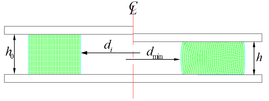
The ring compression in Figure 5.4 is sensitive to friction and is therefore widely used for the purpose of evaluating friction. In ring compression, the changes in the inner and outer diameters of the ring with reduction ratio are greatly influenced by the friction condition, as shown in Figure 5.5. That is, the change in the value \(z = (d_{\text{min}} - d_o)/d_o\) with \(h\) occurs sensitively. As an extreme example, when there is no friction, i.e. in homogeneous ring compression, the ring unconditionally expands. That is, the inner diameter of the ring increases. On the other hand, when the friction is extremely large so that the adhesion condition applies, the inner surface deforms convexly inward. Because of this, the ring compression test is widely used for the purpose of evaluating friction.

Figure 5.4 Ring compression test

(a) μ = 0.1

(b) μ = 0.5

Figure 5.5 Ring compression test and the correlation between friction magnitude and the ring compression process

Using the finite element method for metal forming processes, i.e. metal forming simulation technology, if the relationship curve between the minimum inner diameter and the reduction ratio is constructed according to various friction laws and conditions while the flow stress of the material is fixed, it can be used for the purpose of evaluating friction. This is called the calibration curve of friction.

For example, Figure 5.6 is a friction calibration curve for a material whose flow stress is \(\bar{\sigma} = 503(1+\bar{\varepsilon}/0.05)^{0.26}\) MPa. The ratio of inner diameter : outer diameter : height of the specimen used to obtain this curve is 3 : 6 : 2. Using this curve, the friction coefficient or friction constant can be determined by comparing the experimental curve obtained from the test with this friction calibration curve. The friction calibration curve differs from material to material and differs according to the state of the material. That is, it differs somewhat according to the flow stress used in the analysis of the ring compression test. Figure 5.5 is a friction calibration curve for a strain-rate-independent material. Therefore, there is no need to consider the influence of velocity during the analysis.

Figure 5.6 Friction calibration curve obtained from the analysis results of the room-temperature ring compression test

Figure 5.7 Friction calibration curve obtained from the analysis results of the high-temperature ring compression test

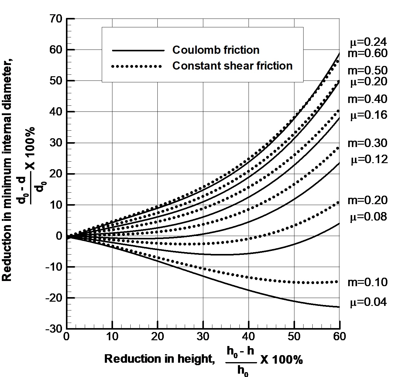
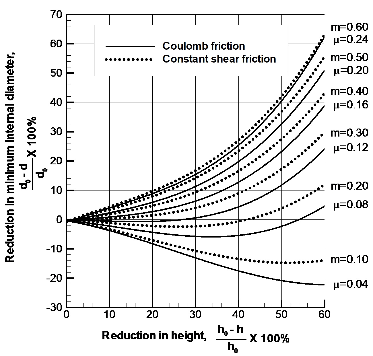
Figure 5.7 is the high-temperature friction calibration curve for the same material. The flow stress at high temperature is \(\bar{\sigma} = 66.0 \dot{\bar{\varepsilon}}^{0.195} \text{MPa}\). To obtain Figure 5.7, the inner diameter, outer diameter, and height of the ring were set to 30 mm, 60 mm, and 20 mm, respectively, and the velocity was assumed to be 200 mm/s. Strictly speaking, the high-temperature friction calibration curve in Figure 5.7 varies not only with the flow stress of the material but also with the velocity.

By carrying out a ring compression test and constructing the curve of the change in the inner diameter at the mid-plane with reduction ratio, the friction coefficient or friction constant can be estimated by comparing it with the friction calibration curve. This is the method of obtaining the friction condition from the ring compression test.

Comparing Figure 5.6 and Figure 5.7, it can be seen that the law of Coulomb friction and the law of constant shear friction show similar patterns, especially at low reduction ratios and low friction. However, at high reduction ratios and high friction, the slopes of the friction calibration curves of the two friction laws show some difference. Of course, this is a result of the influence of the normal stress being reflected in the law of Coulomb friction. From Figure 5.6 and Figure 5.7, it can be seen that the friction constant is approximately twice the friction coefficient.

Meanwhile, on the basis of the friction calibration curve, the law of Coulomb friction and the law of constant shear friction are often perceived as similar. In some cases this is greatly different from the truth (for details, see Section 5.7). The two friction laws are fundamentally bound to be similar if the pressure variation at the contact surface is small. In ring compression, owing to the nature of the hollow material, the friction hill is relatively indistinct. That is, the difference in pressure at the contact surface is not large. This phenomenon is even more evident at low friction. Therefore, just because the two friction laws caused similar ring deformation in ring compression, one cannot say that the two friction laws are similar. Because the pressure distribution on the contact surface in ring compression is relatively small compared with forging and the like, it is only natural that the results predicted by the two friction models are similar. Discussing the relationship between the two frictions from ring compression is in itself not valid.

5.7 Influence of friction law and friction condition

In this section, the aspect ratio of a process is defined as the ratio of the height to the width of the material, and the contact area ratio is defined as (the area of the contact region of the material)/(the area of the entire surface).

(1) Low-aspect-ratio cylinder compression

Figure 5.8 shows the analysis results obtained under identical conditions for a low-aspect-ratio, low-contact-area-ratio cylinder compression process using the law of Coulomb friction and the law of constant shear friction. The process conditions used in this analysis are identical to those used to obtain the friction calibration curve in Figure 5.7. Figure 5.8(a) is for a friction coefficient \(\mu = 0.2\), and Figure 5.8(b) is for a friction constant \(m = 0.48\). The friction coefficient and friction constant used here are mutually corresponding values, as shown in Figure 5.7. As shown in the metal flow lines in Figure 5.8, it can be seen that for the low-aspect-ratio problem the two friction laws predict similar plastic flow lines. This is also the case in terms of forming load, as shown in Figure 5.9.

(a) Law of Coulomb friction (μ = 0.2) (b) Law of constant shear friction (m = 0.48)

Figure 5.8 Comparison of plastic flow lines in low-aspect-ratio and low-contact-area-ratio cylinder compression

Figure 5.9 Comparison of forming loads in low-aspect-ratio and low-contact-area-ratio cylinder compression

(2) High-aspect-ratio cylinder compression process

Figure 5.10 and Figure 5.11 show the analysis results of the high-aspect-ratio cylinder compression process. For this, the same process conditions as those used to obtain the friction calibration curve in Figure 5.7 were used. Figure 5.10(a) is the result using a friction coefficient μ = 0.2, and Figure 5.10(b) is the result using a friction constant μ = 0.48. Figure 5.11 shows the change in forming load. What can be seen simultaneously in these two results is that, although the two friction models predicted similar results at first, the difference in the results widens as the stroke increases. This fact means that as the aspect ratio or contact area ratio increases, the difference between the two friction laws widens.

(a) Law of Coulomb friction (μ = 0.2) (b) Law of constant shear friction (m = 0.48)

Figure 5.10 Comparison of plastic flow lines in high-aspect-ratio and high-contact-area-ratio cylinder compression

Figure 5.11 Comparison of forming loads in high-aspect-ratio and high-contact-area-ratio cylinder compression

(3) Ring gear forging process

A ring gear is a product with a relatively large aspect ratio and contact area ratio. For the finite element analysis of a typical ring gear forging process, a strain-rate sensitivity exponent of 0.195 was used, and the upper die was assumed to descend at a constant velocity of 500 mm/s. A friction coefficient of μ = 0.1 was used, and a friction constant of m = 0.2 was used. Of course, these two friction conditions are mutually corresponding conditions, as shown in Figure 5.12. These conditions differ from the conditions of an actual hot forging process and were merely assumed in order to analyze the difference between the friction laws.

(a) Plastic flow lines

(b) Forming load

Figure 5.12 Comparison of the predicted results of the ring gear forging process according to the friction law

From the results of Figure 5.12, it can be seen that a very large difference exists, especially around the axis of symmetry. This is because the law of constant shear friction causes low friction in the high-pressure region at the central part and causes high friction in the die-material boundary region adjacent to the free surface. The comparison of forming loads in Figure 5.12(b) shows the difference between the two friction laws more clearly. The law of Coulomb friction predicted a forming load about 30% larger than that of the law of constant shear friction.

(4) Cold extrusion of a long billet

Even if the aspect ratio is small, if the contact area ratio is large, friction is not an easy problem. A typical problem can be seen in a multi-stage extrusion process such as that shown in Figure 5.13(a). The flow stress of the material used in this analysis is \(\bar{\sigma} = 50.3(1+\bar{\varepsilon}/0.05)^{0.26}\) MPa, the law of Coulomb friction was used, and the friction coefficient was assumed to be 0.1.

From the analysis result of Figure 5.13(a), i.e. the distribution of the effective strain, it can be seen that, even though the friction coefficient is not a very large value, somewhat abnormal plastic deformation occurred near the punch. Of course, if the corresponding law of constant shear friction is used, this problem does not occur. However, if the container is long and the friction constant in the law of constant shear friction is relatively large, then even if abnormal plastic deformation does not occur around the punch, an excessive forming load may be predicted.

(a) Constant friction coefficient (b) Variable friction coefficient

Figure 5.13 Analysis of a high-extrusion-ratio and long-container forward extrusion process and the law of Coulomb friction

In Figure 5.13(a), the abnormal plastic flow phenomenon is due to the excessive friction stress of the law of Coulomb friction. Of course, the direct cause of this lies in the assumption that the friction coefficient is constant over the entire contact boundary, based on the friction condition at the exit. One way to avoid this problem is to divide the die into several pieces and input a different friction coefficient for each region according to the pressure (normal stress) and the effective strain of the material. In an actual container, since the material and the die are completely separated by the lubricant, the friction coefficient is bound to be small. However, at the exit the situation is exactly the opposite. The lubricant film coated on the material is greatly damaged, and the pressure greatly increases. Taking this into account, if the friction coefficient is determined by intuitively considering the deformation of the lubricant as shown in Figure 5.13(b), abnormal plastic flow does not occur.

However, because of usability issues, this method may not attract the attention of users. For this reason, the hybrid friction law of Eq. (5.6) or the weighted-function friction law using Eq. (5.7) and Eq. (5.8) can be useful. As shown in Figure 5.2, the hybrid friction law follows the law of Coulomb friction \(\sigma_t = -\mu\sigma_n g(v_t - \bar{v}_t)\) when the normal stress is small and follows the law of constant shear friction \(\sigma_t = m'k g(v_t - \bar{v}_t)\) when the normal stress is large. Of course, the limit frictional factor \(m'\) in this case can also be used for the purpose of defining the upper bound of the friction stress, and it need not be regarded as the friction constant \(m\) corresponding to the friction coefficient \(\mu\).

(5) Backward extrusion of a square cup with a high area-reduction ratio

In a three-dimensional analysis, especially if the material is thin as in Figure 5.14(a), the law of Coulomb friction can cause excessive constraint due to the coarse element density in the thickness direction at the bottom, and the law of constant shear friction is also likely to cause the problem of over-constraint at the side-wall surface. In such cases, it is necessary to consider the use of the hybrid friction law. Of course, before using this friction law, the accumulation of experience through comparison with experimental results should precede it. Figure 5.14(b) and Figure 5.14(c) are the results using the law of Coulomb friction and the hybrid friction law, respectively. And as shown in the figures, it can be seen that the through-thickness distribution of elements at the bottom surface is not sufficient. This problem cannot be solved simply by increasing the number of elements. Therefore, the law of Coulomb friction, together with the mesh, can lead to over-constraint. In fact, comparing Figure 5.14(b) and Figure 5.14(c), this fact can be recognized.

In conclusion, the hybrid friction law is useful in backward extrusion processes with a very large extrusion ratio. In this case, it is important to appropriately set the friction coefficient \(\mu\) and the limit frictional factor \(m'\) through comparison of experimental results and analysis results. If the law of constant shear friction is used to solve the aforementioned problem, then once the material that has already exited the main deformation zone comes into geometric contact with the wall surface of the die, it can cause the problem of over-constraint and oscillation of the results.

(a) Backward extrusion process

(b) Coulomb friction (c) Hybrid friction

Figure 5.14 Analysis of a square cup backward extrusion process with a high area-reduction ratio

(6) Treatment of the fracture surface in automatic multi-stage cold forging

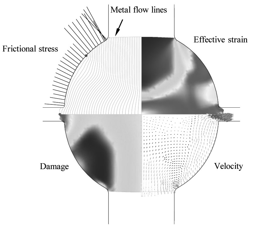
In cold forging, a phosphate coating or a molybdenum disulfide (\(\text{MoS}_2\)) coating is generally applied to the surface of the material for lubrication purposes. And in press forging, annealing heat treatment is carried out when the deformation is severe, and the coating treatment is reapplied each time. However, in automatic multi-stage forging, coated coil material is used, and the cross-section cut in the forging machine cannot be coated. Of course, for this reason, automatic multi-stage forging is carried out in an atmosphere of lubricating oil. In any case, the fracture surface and the side surface are bound to differ greatly in terms of friction. Therefore, for problems in which friction is important, it is necessary to input different friction coefficients for the fracture surface and the side surface. As shown in Figure 5.15, it can be seen that the friction stress differs according to position owing to the different friction coefficients. In the figure, the length of the vertical line segment denotes the magnitude of the friction stress.

Figure 5.15 Steel ball manufacturing process – the case where the friction stress differs from position to position

(7) Simultaneous expansion and reduction process of a long pipe

The simultaneous expansion and reduction process of a long thin pipe in Figure 5.16 is sensitive to the friction law. This is because the normal stress at the die-material contact surface is relatively small, whereas the contact region is large. In this process, the upper and lower ends of the pipe are formed simultaneously. The upper part is expanded, and the lower part is reduced. If the friction is large, the radius of the middle part of the pipe increases, and contact between the material and the die will occur at the middle part. In this case, since the contact region is large, the plastic flow of the material is bound to be greatly affected by the friction law and the friction condition.

The flow stress used in the analysis of this process is \(\bar{\sigma}=617.0\bar{\varepsilon}^{0.25}\) MPa. The process analysis was carried out under the two friction laws and various friction conditions. The friction constant corresponding to the friction coefficient was obtained from Figure 5.6 (although the material is different, there is no significant difference because the work-hardening exponent is similar). Selecting one of the analysis conditions, the deformed shape is shown in Figure 5.17. To quantitatively evaluate the effect of the two friction laws, the protrusion length \(d\) in Figure 5.16(b) was examined, and the results are summarized in Figure 5.18. From this figure, one arrives at the conclusion that, for this example, there is no similarity between the two friction models. The point to be emphasized here is the fact that the law of constant shear friction imposes excessive friction stress even in regions that are mechanically separated but geometrically in contact, and is therefore likely to produce a relatively large difference from actual phenomena. This is the problem that was also of concern in the backward extrusion of a square cup with a high area-reduction ratio described earlier.

(a) Initial          (b) Final

(a) μ = 0.05          (b) m = 0.096

Figure 5.16 Simultaneous reduction/expansion process of a long pipe

Figure 5.17 Example of predicted results

Figure 5.18 Change in protrusion length d with friction

In conclusion, when friction is relatively unimportant in a process or when the variation of the normal stress is small, the law of Coulomb friction and the law of constant shear friction are similar, but in metal forming processes where friction is important, the two friction laws have no similarity. Therefore, it is recommended to use the law of Coulomb friction whenever possible and, depending on the case, to selectively use the hybrid friction law or the weighted-function friction law. In particular, since the number of meshes is constrained in three-dimensional analysis, the predicted results of the friction phenomenon can be relatively greatly affected by the mesh, so it is worthwhile to actively consider the use of the hybrid friction law.