14 Metal Forming Simulation
14.1 Accuracy of Results
The analysis results concerning macroscopic phenomena include everything mentioned in plasticity theory. Deformed shape, temperature distribution, stress and effective stress, hydrostatic pressure, strain rate and effective strain rate, effective strain, velocity field, wear index, damage index, grain flow lines, forming load, and the principal directions and magnitudes of stress and strain rate belong to the main results.
The most suitable method for verifying analysis results is the comparison of grain flow lines. A grain flow line refers to the result of tracking a grid of the direction and size that the user desires. In general, the base material is manufactured by rolling and drawing processes, and in this process a grain is formed in the longitudinal direction due to the directional deformation of the crystals. When a forging material is cut, polished, and then etched, corrosion occurs first at the grain boundaries, so that the grain formed in the longitudinal direction is visualized. By comparing the grain thus obtained, that is, the grain flow lines, with the predicted grain flow lines, the validity of the analysis results can be verified.
The forming load and the like are also sometimes used for the purpose of validating analysis results, but it is difficult for them to have more than qualitative meaning. This is because the analysis result of the forming load can differ by more than 20% depending on whether or not the elastic deformation of the die is considered [14.1], and because it is not easy to quantitatively compare flow stress and friction.
14.1.1 Hot Forging
The example in Figure 14.1 is a case where the external shape was successfully formed but the process design failed because of a defect in the grain flow lines, that is, an internal defect, and it emphasizes the importance of controlling grain flow lines in forging process design [11.7].
An isothermal analysis was performed, and the process conditions and the flow stress of the material used are as follows.
Die velocity: \(\bar{V}_D = 300\) mm/s ; Friction coefficient: \(\mu = 0.3\) ; Flow stress: \(\bar{\sigma} = 62.0 \bar{\varepsilon}^{0.18}\) MPas
Figure 14.1 shows the process of change of the metal flow lines. The metal flow lines at the inner lower part of the final product form a deep valley. The surface of this part is machined by cutting, and in this process a discontinuity of the grain flow lines occurs, degrading the surface characteristics and strength. Therefore, this example is a typical case where the forming of the external shape was successful but it failed due to a defect in the grain flow lines.
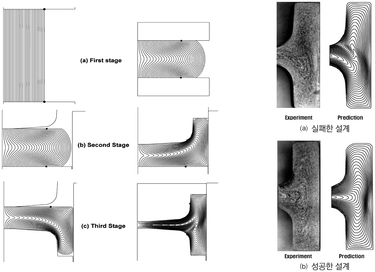
Figure 14.2(a) compares the experimental results and the analysis results. It can be confirmed that the two results agree well. Figure 14.2(b) compares the analysis results and experimental results for a good product obtained by an improved process design. This figure emphasizes the importance of metal forming simulation technology in developing a process in which restrictions on the internal metal flow lines are imposed.
Figure 14.3 shows the analysis results of the hammer forging of a crankshaft for a medium-sized ship engine. This process is a case where, because the size of the die is very large, the development cost and development period are considerable, so that the loss due to process design failure becomes an issue. The purpose of analyzing this process is, together with the presence or absence of external defects, the time required for forging, that is, the number of blows of the hammer press. As seen in the figure, it can be seen that the external analysis result agrees well with the experimental result [14.2].
Figure 14.4 compares the predicted grain flow lines and experimental results of the axisymmetric hot closed-die forging process of an automobile part. From the figure, it can be confirmed that the predicted grain flow lines for the two examples well reflect the experimental results.
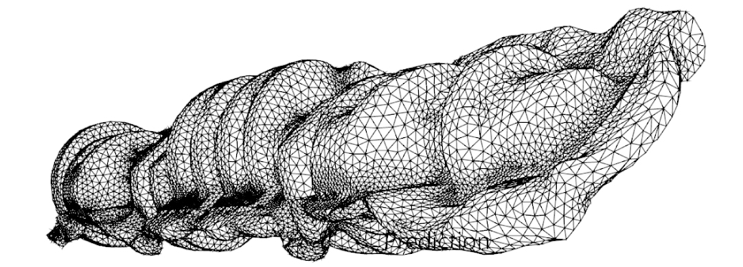
(a) Predicted result
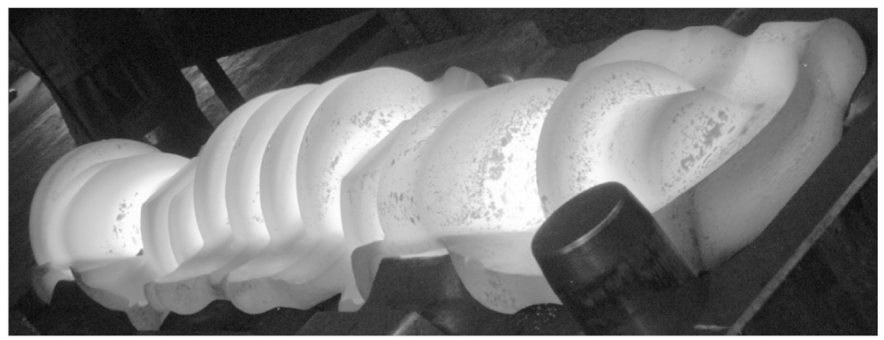
(b) Experimental result
Figure 14.3 Comparison of analysis and experimental results of the hammer forging process [14.2]
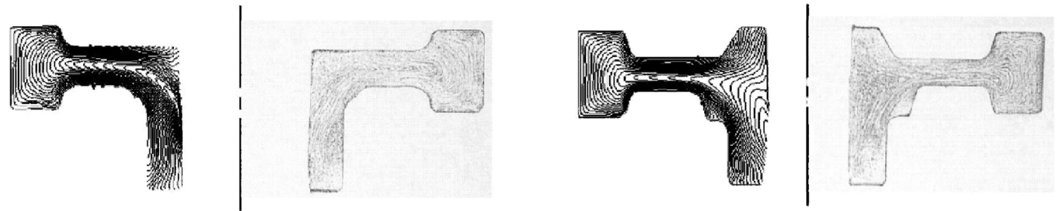
Figure 14.4 Analysis and experiment of the hot closed-die forging process of gear blanks [14.3]
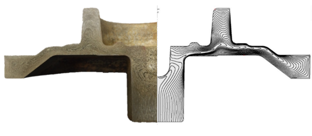
Figure 14.5 Analysis and experiment of the hot closed-die forging process of an automobile part [14.4]
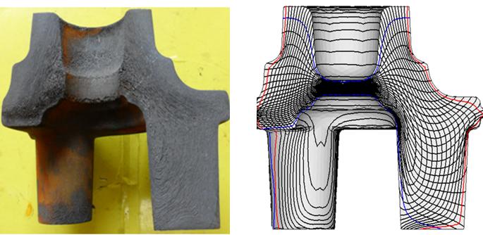
Figure 14.6 Analysis and experiment of the hot closed-die forging process of a planetary gear part [14.5]
14.1.2 Cold Forging
Figure 14.7 compares the analysis results and experimental results of a 5-stage axisymmetric cold forging (automatic multi-stage cold forging). Although the final product shape of this process appears relatively simple, it is in fact a complex process requiring precise analysis. As seen in the figure, in terms of the final product shape the predicted results and the experimental results agree engineeringly.
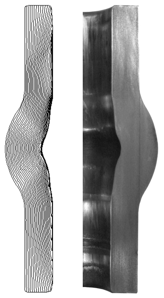
Figure 14.7 Comparison of predicted and experimental results
Figure 14.8 compares the analysis results and experimental results of the extrusion process of two materials, namely SCM435 and ESW105. A friction coefficient of 0.03 was used, and the flow stress of Figure 12.9(b) was used. For both materials the analysis results and experimental results are similar. In particular, in the case of SCM435, in both the analysis results and the experimental results the workpiece contacts the outer wall of the extrusion container, whereas for ESW105 it is the opposite.
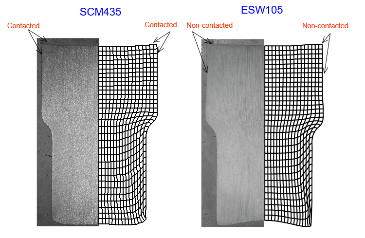
Figure 14.8 Comparison of predicted and experimental results of the extrusion process [14.6]
The Baden-Baden benchmark test problem [14.7, 14.8] has been studied by many experts. This problem is a 2-stage cold forging process as seen in Figure 14.9, and although it is a simple process in appearance, from the standpoint of the analysis engineer it belongs to somewhat tricky problems. Because the corner of the lower part is progressively crushed in the first stage and the upper die simultaneously contacts the upper part of the workpiece at the start of the second stage, quality control of the mesh is not easy. For this reason, the research results by most researchers showed a large difference in the left and right heights compared with the experimental results, and a result in which the internal characteristic boundary is severely crushed was caused.
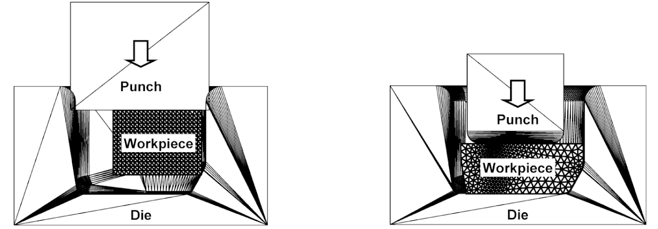
Figure 14.9 Baden-Baden benchmark test problem
Die velocity: \(\bar{V}_D = 300\) mm/s ; Friction coefficient: \(\mu = 0.3\) ; Flow stress: \(\bar{\sigma} = 62.0 \bar{\varepsilon}^{0.18}\) MPa
The predicted results are shown in Figure 14.10 and Figure 14.11. As seen in Figure 14.10(a), it can be seen that especially in the first stage the element density well reflects the die-workpiece boundary. In the second stage as well, the boundary between the die and the workpiece is well reflected in the element density, and as a result this appeared as the effect of well expressing the upper internal boundary, that is, the characteristic boundary, as seen in Figure 14.10(b). It can be confirmed that the corners are well expressed despite the fact that the number of elements is not large. This is an essential element in precise metal forming simulation.
Meanwhile, if the ratio of the left and right lengths defined in Figure 14.11 is calculated, about 20.0% is obtained. This value is relatively close to the experimental result [14.8].
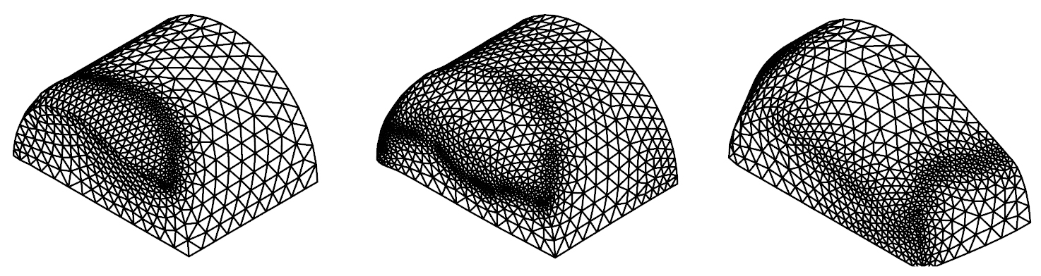
(a) Stage 1
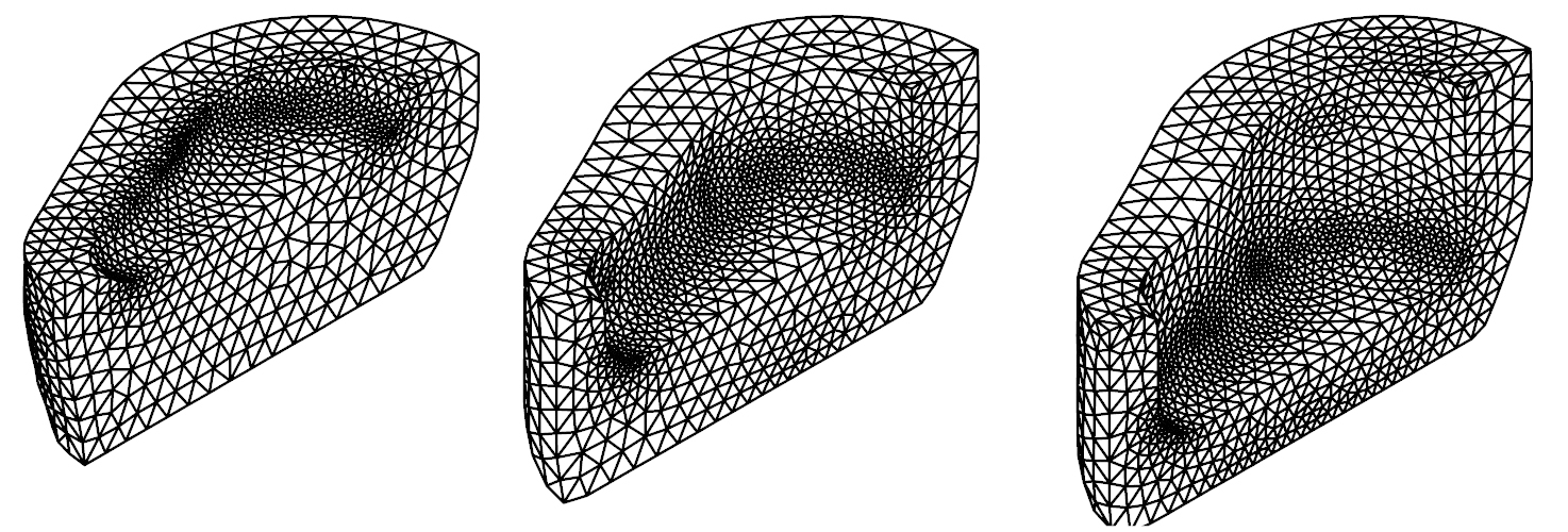
(b) Stage 2
Figure 14.10 Predicted results emphasizing the mesh density
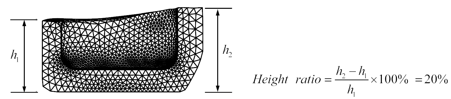
Figure 14.11 Comparison of left and right heights
Figure 14.12 compares the analysis results and experimental results of a three-dimensional cold forging process. Figure 14.12(a) compares the ovality formed during piercing by a circular punch in the pinch-yoke cold forging process. It falls within an error range that can be qualitatively accepted. Figure 14.12(b) compares the analysis results and experimental results of the rotor-pole cold forging process. At the main points of interest the predicted results well reflect the experimental results.
Figure 14.12(c) compares the analysis results and experimental results of the yoke automatic multi-stage cold forging process. In this process the control of springback is very important. It is a case where successful process development was achieved based on the prediction results of springback [14.9].
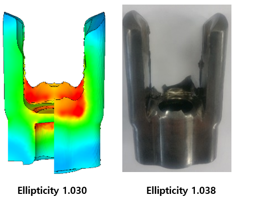
(a) Pinch-yoke forging process
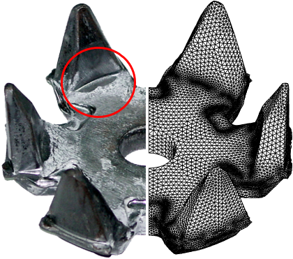
(b) Rotor-pole forging process
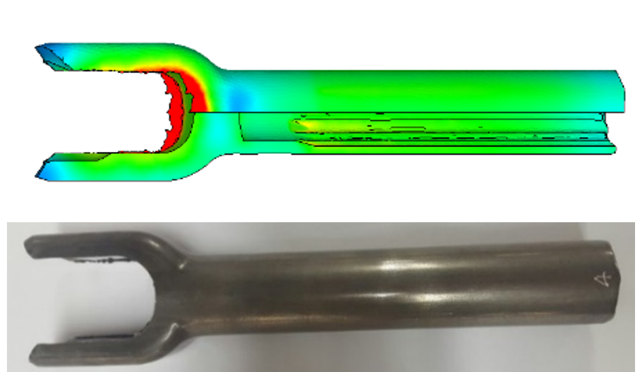
(c) Yoke forging process
Figure 14.12 Cases of comparison of predicted and experimental results of cold forging
14.2 Summary of Factors Affecting the Results
First, let us examine the mechanical factors. How to view the deformation of the material is the largest element.
The flow stress of the workpiece can generate plastic flow with a relatively large difference at parts where local underfilling problems occur or where deformation occurs severely and locally. In cold forging, the strain-hardening exponent in the flow stress is the factor that has the greatest influence on identifying the causes of local defects, buckling, and internal and external cracks.
In cold forging, low-friction regions are generally widely distributed. In particular, in forward and backward extrusion, the material that has passed through the die exit often only maintains a geometrical contact state. In such problems the constant shear friction law can cause excessive friction. Currently many application engineers tend to use the constant shear friction law, but it is recommended to use the Coulomb friction law as much as possible. There is also research that discusses wear using constant shear friction, but this is an extreme case of misuse.
The fracture of materials is explained by ductile fracture and brittle fracture. Since cold forging materials generally belong to ductile materials, the fracture phenomenon of the material during forging is explained by ductile fracture theory. In ductile fracture theory, fracture occurs when the damage accumulated in the material reaches the critical damage. On the other hand, in brittle fracture, when the maximum principal stress reaches a certain magnitude, fracture occurs on the plane perpendicular to the maximum principal stress axis.
Although the initial material of cold forging belongs to ductile materials, as the material undergoes deformation the effective strain accumulates and it tends to become brittle, so in predicting the fracture surface, ductile fracture should be considered as the center while brittle fracture should also be considered at the same time. Damage is known not only to have a direct influence on fracture but also to have some influence on flow stress. Some researchers have attempted a solution by coupling ductile fracture theory with flow analysis, but it is considered that the influence of damage on flow stress is negligible in normal processes. The critical damage has an important influence on judging the fracture of the material, and it is empirically necessary to devote great effort to the accumulation of critical damage values. In the hot state, it is important to know the range of the hot-shortness temperature. This is because if forging is carried out in this range, severe internal cracks are left behind.
In addition to the mechanical factors explained above, there are numerical factors that directly affect the finite element prediction results. First, the number of elements can be mentioned. It is common knowledge that increasing the number of elements increases the accuracy of the solution. However, in the simulation of metal forming problems that entail remeshing, the situation is different. Remeshing inevitably causes smoothing of the state variables, and frequent remeshing becomes a factor that lowers the accuracy of the analysis results. This is because, when the number of elements increases, the size of the elements in the main deformation region becomes smaller, and local deformation occurs as a result. Since this leads to remeshing, a somewhat large number of elements becomes a factor that lowers the accuracy of the results. Therefore, it is desirable to use an appropriate number of elements.
In general, it is assumed that there is no volume change during metal forming. This assumption is formulated as an incompressibility condition, and two methods are used to handle it. These are the Lagrange multiplier method and the penalty method. In the Lagrange multiplier method, the hydrostatic pressure becomes an unknown, so the number of unknowns increases, whereas in the penalty method the incompressibility condition is enforced without adding variables. Therefore, the Lagrange multiplier method takes relatively more computation time but has the advantage of higher accuracy of results and the elimination of numerical problems. Therefore, if the Lagrange multiplier method is provided, using this function is advantageous from the standpoint of accuracy of the solution and numerical stability.
Metal forming simulation is summarized as repeating the operation of, at the present point in time, obtaining the movement velocities of the nodes that satisfy the mechanical principles and geometrical conditions, and then moving the nodes in a fixed direction over a certain time increment. At this time, if the time increment is kept at the input fixed value, some nodes may penetrate the die, or workpiece nodes on the die may separate from the die. When a workpiece node penetrates the die, the workpiece that has penetrated the die must be removed, or the workpiece must be pushed onto the die surface. This process proceeds frequently in the actual simulation process, and it has some influence on the analysis results. Therefore, the average time increment calculated from the input information must be reasonably determined, and appropriately sized die-penetration limits and die-separation limits of the workpiece must be input. These values are major numerical factors that are directly connected to the volume change rate and the like of the analysis results.
Meanwhile, in the rigid-plastic finite element method, in the plastic flow rule related to the von Mises (or Huber-von Mises) yield theory, \(\sigma'_{ij} = (2\bar{\sigma}/3\dot{\bar{\varepsilon}})\dot{\varepsilon}_{ij}\), when \(\dot{\bar{\varepsilon}}\) approaches zero, the computation becomes numerically impossible. Therefore, a lower limit of the effective strain rate \(\dot{\bar{\varepsilon}}\) must be set. In general, if this value is made larger than normal, the acquisition of the solution is easy, but depending on the problem it has some influence on the accuracy of the results. Conversely, if this value is made smaller than normal, it clarifies the distinction between the elastic region and the plastic region and can minimize the artificial plastic deformation of the elastic region, but much effort is required to obtain the solution, and in this process the accuracy of the solution may worsen.
In the rigid-plastic finite element method, it is assumed that there is no change in volume during metal forming. In other words, as in fluid mechanics, an incompressibility condition is attached. However, actual metal forming simulation inevitably accompanies volume change. Its causes can be broadly divided into three. The first stems from theory, namely the handling technique of the incompressibility condition. The incompressibility condition is usually handled by the Lagrange multiplier method and the penalty method, and among these the penalty method handles the incompressibility condition approximately, so depending on the penalty constant it causes a slight volume change. Moreover, a very large penalty constant causes uncertainty of partial plastic flow. For example, in a two-dimensional axisymmetric problem, it can produce results of low reliability around the central axis. Therefore, it is desirable to use the Lagrange multiplier method as much as possible. Of course, the Lagrange multiplier method accompanies an increase in the number of unknowns. In the case of a two-dimensional quadrilateral mesh, an increase in unknowns equal to the number of elements occurs, and in the case of a three-dimensional tetrahedral mesh, an increase in unknowns equal to the number of nodes occurs. Therefore, when analyzed with the same elements, the Lagrange multiplier method is advantageous in terms of accuracy but disadvantageous in terms of computation time.
The second volume-change factor is due to the updating of the velocity field, that is, the advancement of the nodes by the product of the velocity field and the time increment, and it is related to the solution method of the forging process. The analysis of forging and other metal forming processes is a repetition of the process of obtaining the velocity field at one instant and advancing it by the time increment the user has input. In the implicit method, the velocity field for one instant around the middle part of the time increment is obtained, and then the nodes are advanced, thereby calculating the deformed shape step by step. On the other hand, in the explicit method, the velocity field at the start point of the time increment is calculated. Therefore, basically in the explicit method many variables are already determined, so it is advantageous in terms of computation time and acquisition of the solution, but compared with the implicit method it is greatly disadvantageous in terms of accuracy, volume change, and the like. In the implicit method on which AFDEX is based, there is the advantage that the time increment can be made relatively large, but it is necessary to remember the fact that the larger this value is made, the larger the volume change becomes. As a countermeasure to this second factor, the best path is to accumulate direct and indirect experience regarding volume change through the repetition of the process of analyzing the extrusion process and the upsetting process without using the volume-compensation function and then checking the volume change rate.
The third volume-change factor is remeshing, whose cause lies in numerical aspects. In the finite element method, the shape of the workpiece is basically defined by the connection of the nodes on the outline or surface. Therefore, remeshing inevitably accompanies volume change. In particular, in three dimensions, because the die is generally cylindrical, the volume tends to become smaller as the number of elements becomes smaller. Therefore, it can be said that the volume is sensitively affected by remeshing. For this problem too, the solution depends on the empirical factors of the user and the degree of intelligence of the software.
Comprehensively speaking, volume change is directly connected to the reliability of the predicted results, and it is a matter to which the user must always pay attention. As mentioned above, most commercial software provides a function for artificial compensation of the volume change that unavoidably occurs during analysis, but it is emphasized that relying on this uncritically is not an appropriate solution. Insight into volume change and the technique for dealing with it are among the core knowledge and skills that a user must possess. In cold forging, the plastic flow of the workpiece is not greatly affected by velocity. However, although the degree differs depending on the process, what is clear is the fact that there is some degree of influence. According to the experience of engineers involved in automatic multi-stage cold forging that is actually produced at high speed, the fact that there is some influence of velocity cannot be ignored. However, unless it is a special process such as ultra-high-speed production, a realistic approach would be to predict while ignoring the influence of velocity and then reflect the influence of velocity empirically. Of course, when the influence of velocity has been quantified experimentally, it is not difficult to consider that influence using Equation (2.128) or a similar flow stress equation model.