4 Hooke's Law and the Plastic Flow Rule

4.1 Tensile test

The tensile test is widely used for the purpose of characterizing the macroscopic properties of a material. Figure 4.1 is a typical example of the tensile test curve for a metal bar at room temperature. The horizontal axis is the increase in the gauge length \(\Delta l\) divided by the initial distance between gauge marks \(l_0\), i.e. the nominal strain (engineering strain) \(\varepsilon_e\), and the vertical axis is the current load \(P\) divided by the initial cross-sectional area \(A_0\), i.e. the nominal stress (engineering stress) \(\sigma_e\).

In the tensile test curve, the maximum nominal stress is called the tensile strength \(\sigma_u\), and the maximum nominal strain (\(\varepsilon_F\)) \(\times 100(\%)\) is called the elongation. The nominal stress \(\sigma_Y\) corresponding to the point \(Y\) at which initial yielding occurs is called the initial yield stress or the yield strength. When the nominal stress \(\sigma_e\) and the nominal strain \(\varepsilon_e\) are in a linear proportional relationship, the material is said to be linear elastic, and the limiting nominal stress is called the proportional limit. The slope \(E\) of the straight line is called the modulus of elasticity or Young's modulus. From an engineering standpoint, it is acceptable to regard the range from the proportional limit up to initial yielding as the nonlinear elastic region.

(OP: linear elastic, PY: nonlinear elastic, YF: plastic)

Figure 4.1 Nominal stress versus nominal strain curve

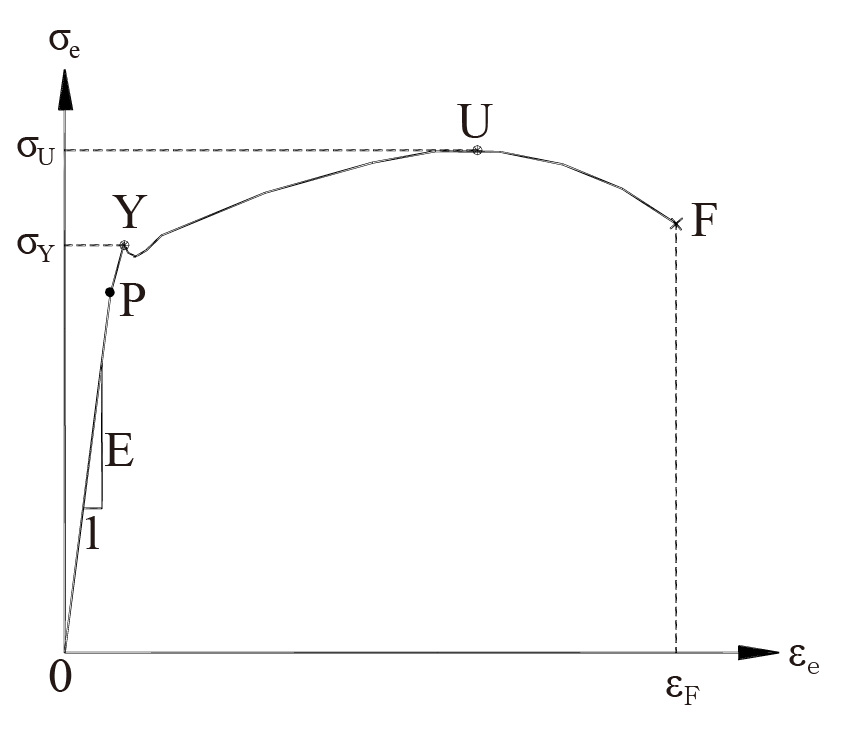
During the tensile test the specimen does not elongate uniformly; instead, a localized plastic deformation region migrates and the specimen elongates progressively. When a certain region undergoes plastic deformation, its cross-section shrinks and, accordingly, the stress per unit area increases. Therefore, from the mechanical, i.e. stress, viewpoint, the region that deforms first and whose cross-section is reduced is the weakest. However, when plastic deformation occurs, dislocations are generated, and in general, as the dislocation density increases, the material develops a resistance to deformation so that its load-bearing capacity actually increases. If the increase in load-bearing capacity due to deformation resistance is greater than the decrease in load-bearing capacity due to the cross-sectional reduction, the plastic region moves elsewhere. Conversely, if the decrease in load-bearing capacity due to the cross-sectional reduction becomes greater than the increase due to deformation resistance (in general, the rate of increase of the deformation-resistance capacity decreases as deformation increases), the tensile specimen enters an unstable state, and continued deformation occurs in the region weakened by the cross-sectional reduction. That is, necking occurs, leading to fracture. Since the maximum load acts at this point, the maximum nominal stress point is regarded as the onset point of necking. When predicting the location of necking in a tensile specimen mechanically, a unique solution cannot be obtained. Therefore, necking belongs to a class of instability problems (bifurcation problems). At the point where necking begins, the maximum nominal stress, i.e. the tensile strength, is reached.

In general, tensile test results give the relationship between nominal stress and nominal strain. Actual mechanical analysis, however, requires the relationship between true stress and true strain.

Since the nominal strain \(\varepsilon_e\) and the true strain \(\varepsilon_t\) are defined respectively as

\[ \varepsilon_e = \frac{l - l_0}{l_0} = \frac{\Delta l}{l_0} \tag{4.1} \]

\[ \varepsilon_t = \log_e \frac{l}{l_0} = \log_e \left( 1 + \frac{\Delta l}{l_0} \right) \tag{4.2} \]

the following relationship holds between the nominal strain and the true strain.

\[ \varepsilon_t = \log_e (1 + \varepsilon_e) \tag{4.3} \]

In Eq. (4.1) and Eq. (4.2), \(l\) denotes the current gauge length during the tensile test. Meanwhile, the nominal stress \(\sigma_e\) and the true stress \(\sigma_t\) are defined as follows.

\[ \sigma_e = \frac{P}{A_0} \tag{4.4} \]

\[ \sigma_t = \frac{P}{A} \tag{4.5} \]

where \(A\) is the current cross-sectional area during the tensile test. Since the volume change of a metallic material during plastic deformation is negligibly small, if it is neglected, the following condition holds between the yield point and the onset point of necking.

\[ l_0 A_0 = l A \tag{4.6} \]

From Eqs. (4.4), (4.5), and (4.6), the following relationship can be derived.

\[ \sigma_t = \frac{P}{A_0} \frac{A_0}{A} = \sigma_e(1+\varepsilon_e) \tag{4.7} \]

In this book, the stress \(\sigma\) and the strain \(\varepsilon\) without a trailing subscript \(e\) denote the true stress \(\sigma_t\) and the true strain \(\varepsilon_t\), respectively.

Let us consider the tensile test curve together with the intended use of the material. The stress in a structural material must remain around the point \(O\) during the operation of the structure. Since a safety factor \(S\) is taken into account when designing a structure, the actual usable range is within \(\sigma < \sigma_Y / S\). In metal forming, the material is shaped by relying on plastic deformation, so plastic deformation is the primary concern. Of course, in metal forming, elastic deformation such as springback is often an issue, but the forming process itself relies on plastic deformation. These two cases correspond to states far away from \(Y\). However, for design purposes there are also cases in which the state is deliberately kept around \(Y\), i.e. cases that simultaneously involve elasticity, plasticity, and fracture. Mechanical safety devices and can openers belong to this category.

The tensile test described above pertains to a bar in which directionality in the circumferential direction can be neglected. Sheet material is somewhat more complex because its directionality cannot be neglected. However, since sheet material mostly permits small-thickness deformation using stretching, i.e. deformation up to the point before necking, the deformation after necking is not regarded as important.

4.2 Hooke's law

Hooke's law (De potentia restitutiva (1678) by R. Hooke) states that when a force is applied to a body, a linear proportional relationship holds between the elongated length and the force. Taking as an example a spring with spring constant \(k\), the elongated length \(\delta\) is related to the force \(P\) as follows.

\[ \delta = \frac{P}{k} \quad \text{or} \quad P = k\delta \tag{4.8} \]

A bar or a tensile specimen is also a kind of spring. From a mechanical viewpoint, there is essentially no difference between a bar and a spring. In the tensile test curves of most structural materials, there is a clearly identifiable region in which the elongation of the tensile specimen and the load can be regarded as varying linearly, i.e. a region where Hooke's law applies. That is the segment \(OP\) in Figure 4.1. In this region, the difference between nominal stress and true stress, and between nominal strain and true strain, is small, so they are assumed to be identical. This assumption is the starting point of linear elasticity. From the stress-strain curve in Figure 4.1, Hooke's law under uniaxial loading is expressed as follows.

\[ \sigma = E\varepsilon \quad \text{or} \quad \sigma_{xx} = E\varepsilon_{xx} \tag{4.9} \]

Therefore, Hooke's law is the constitutive equation that expresses the load-deformation characteristics of the segment \(OP\) in Figure 4.1, i.e. of the linear elastic region. The general form of Hooke's law is expressed as

\[ \sigma_{ij} = \sum_{k=1}^{3} \sum_{l=1}^{3} C_{ijkl}\varepsilon_{kl} \tag{4.10} \]

Here, \(C_{ijkl}\) are the elastic constants, a fourth-order tensor quantity composed of a total of 81 components. Since stress and strain are symmetric,

\[ C_{ijkl} = C_{jikl}, \quad C_{ijkl} = C_{ijlk} \tag{4.11} \]

holds. From these conditions, the number of independent elastic constants is reduced to 36. Meanwhile, for a strain-energy density function that is independent of the deformation path to exist,

\[ C_{ijkl} = C_{klij} \tag{4.12} \]

must be satisfied, and from this condition only 21 independent variables remain. Eq. (4.12) is equivalent in meaning to Maxwell's reciprocal theorem. If the material is elastically symmetric with respect to a certain direction, the number of elastic constants is further reduced. For example, when one plane of symmetry exists, it is reduced to 13, and when three planes of symmetry exist (orthotropic material), it is reduced to nine. In the case of a transversely isotropic material, in which every plane containing a single axis is a plane of symmetry and all other planes are asymmetric, the number of elastic constants is reduced to five, and for an isotropic material, in which every plane is a plane of symmetry, the number of elastic constants is reduced to two, namely the modulus of elasticity \(E\) and Poisson's ratio \(\nu\).

In elasticity, loads are classified into mechanical loads and thermal loads. When the temperature of a metal rises, thermal expansion occurs. Therefore, the deformation of a body appears as a combination of deformation due to mechanical loads and deformation due to thermal loads. Of course, in elasticity it is assumed, under the assumption of small deformation, that the two kinds of deformation occur independently. Accordingly, Hooke's law for an isotropic material is summarized as follows.

\[ \begin{aligned} \varepsilon_{xx} &= \frac{1}{E}[\sigma_{xx} - \nu(\sigma_{yy} + \sigma_{zz})] + \alpha\Delta T \\ \varepsilon_{yy} &= \frac{1}{E}[\sigma_{yy} - \nu(\sigma_{zz} + \sigma_{xx})] + \alpha\Delta T \\ \varepsilon_{zz} &= \frac{1}{E}[\sigma_{zz} - \nu(\sigma_{xx} + \sigma_{yy})] + \alpha\Delta T \\ \varepsilon_{xy} &= \frac{(1+\nu)}{E} \sigma_{xy} \\ \varepsilon_{yz} &= \frac{(1+\nu)}{E} \sigma_{yz} \\ \varepsilon_{zx} &= \frac{(1+\nu)}{E} \sigma_{zx} \end{aligned} \tag{4.13} \]

Here, \(E, \nu, \alpha\) are the modulus of elasticity, Poisson's ratio, and coefficient of thermal expansion, respectively, and \(\Delta T = T - T_0\) is the temperature change. Poisson's ratio is the negative of the ratio between the axial normal strain and the lateral strain within the linear elastic range in a tensile test, and theoretically Poisson's ratio must satisfy \(-1 \le \nu \le 0.5\).

If there is no thermal deformation, Hooke's law tells us that the properties of a linear isotropic material are determined by \(E\) and \(\nu\). Meanwhile, rearranging Eq. (4.13) with respect to stress gives

\[ \sigma_{ij} = 2\mu\varepsilon_{ij} + \lambda \sum_{k=1}^{3} \varepsilon_{kk}\delta_{ij} - (3\lambda + 2\mu)\alpha\Delta T\delta_{ij} \tag{4.14} \]

Here,

\[ \mu = \frac{E}{2(1+\nu)}, \quad \lambda = \frac{\nu E}{(1+\nu)(1-2\nu)} \tag{4.15} \]

are called the Lamé constants. In Eq. (4.14), the relationship between stress \(\sigma_{ij}\) and strain \(\varepsilon_{ij}\) is often expressed in the following form.

\[ \sigma_{i} = \sum_{j=1}^{6} D_{ij}\varepsilon_{j} \tag{4.16} \]

Here, the elasticity matrix \(\mathbf{D}\), the stress tensor vector \(\sigma_i\), and the strain tensor vector \(\varepsilon_i\) are defined as follows.

\[ \mathbf{D} = \frac{E(1-\nu)}{(1+\nu)(1-2\nu)} \begin{bmatrix} 1 & \gamma & \gamma & 0 & 0 & 0 \\ \gamma & 1 & \gamma & 0 & 0 & 0 \\ \gamma & \gamma & 1 & 0 & 0 & 0 \\ 0 & 0 & 0 & \beta & 0 & 0 \\ 0 & 0 & 0 & 0 & \beta & 0 \\ 0 & 0 & 0 & 0 & 0 & \beta \end{bmatrix}, \quad \sigma_i = \begin{bmatrix} \sigma_{xx} \\ \sigma_{yy} \\ \sigma_{zz} \\ \sigma_{xy} \\ \sigma_{yz} \\ \sigma_{zx} \end{bmatrix}, \quad \varepsilon_i = \begin{bmatrix} \varepsilon_{xx} \\ \varepsilon_{yy} \\ \varepsilon_{zz} \\ 2\varepsilon_{xy} \\ 2\varepsilon_{yz} \\ 2\varepsilon_{zx} \end{bmatrix} \tag{4.17} \]

Here,

\[ \gamma = \nu / (1-\nu), \quad \beta = (1-2\nu) / 2(1-\nu) \tag{4.18} \]

It is necessary to organize Hooke's law for plane-stress, plane-strain, and axisymmetric problems. Let us first derive the constitutive equation for plane stress. Since \(\sigma_{zz} = \sigma_{zx} = \sigma_{zy} = 0\) in plane stress, substituting this condition into Eq. (4.13) and rearranging gives

\[ \begin{aligned} \varepsilon_{xx} &= \frac{1}{E}(\sigma_{xx} - \nu\sigma_{yy}) \\ \varepsilon_{yy} &= \frac{1}{E}(\sigma_{yy} - \nu\sigma_{xx}) \\ \varepsilon_{zz} &= -\frac{\nu}{E}(\sigma_{xx} + \sigma_{yy}) \\ 2\varepsilon_{xy} &= \frac{2(1+\nu)}{E}\sigma_{xy} \end{aligned} \tag{4.19} \]

and rearranging this equation with respect to the stress tensor vector gives the following.

\[ \begin{bmatrix} \sigma_{xx} \\ \sigma_{yy} \\ \sigma_{xy} \end{bmatrix} = \frac{E}{1-\nu^2} \begin{bmatrix} 1 & \nu & 0 \\ \nu & 1 & 0 \\ 0 & 0 & (1-\nu)/2 \end{bmatrix} \begin{bmatrix} \varepsilon_{xx} \\ \varepsilon_{yy} \\ 2\varepsilon_{xy} \end{bmatrix} \quad \text{or} \quad \sigma_i = D_{ij}\varepsilon_j \tag{4.20} \]

Here, \(\mathbf{D}\), \(\sigma_i\), \(\varepsilon_i\) are defined respectively as follows.

\[ \mathbf{D} = \frac{E}{1-\nu^2} \begin{bmatrix} 1 & \nu & 0 \\ \nu & 1 & 0 \\ 0 & 0 & (1-\nu)/2 \end{bmatrix}, \quad \sigma_i = \begin{bmatrix} \sigma_{xx} \\ \sigma_{yy} \\ \sigma_{xy} \end{bmatrix}, \quad \varepsilon_i = \begin{bmatrix} \varepsilon_{xx} \\ \varepsilon_{yy} \\ 2\varepsilon_{xy} \end{bmatrix} \tag{4.21} \]

Similarly, the equations corresponding to Eq. (4.20) and Eq. (4.21) in plane strain are as follows.

\[ \begin{bmatrix} \sigma_{xx} \\ \sigma_{yy} \\ \sigma_{xy} \end{bmatrix} = \frac{E(1-\nu)}{(1+\nu)(1-2\nu)} \begin{bmatrix} 1 & \nu/(1-\nu) & 0 \\ \nu/(1-\nu) & 1 & 0 \\ 0 & 0 & (1-2\nu)/2(1-\nu) \end{bmatrix} \begin{bmatrix} \varepsilon_{xx} \\ \varepsilon_{yy} \\ 2\varepsilon_{xy} \end{bmatrix} \tag{4.22} \]

\[ \mathbf{D} = \frac{E(1-\nu)}{(1+\nu)(1-2\nu)} \begin{bmatrix} 1 & \nu/(1-\nu) & 0 \\ \nu/(1-\nu) & 1 & 0 \\ 0 & 0 & (1-2\nu)/2(1-\nu) \end{bmatrix} \tag{4.23} \]

In an axisymmetric problem, the only nonzero strain components are \(\varepsilon_{rr}\), \(\varepsilon_{\theta\theta}\), \(\varepsilon_{zz}\), \(\varepsilon_{rz}\), and the only nonzero stress components are \(\sigma_{rr}\), \(\sigma_{\theta\theta}\), \(\sigma_{zz}\), \(\sigma_{rz}\). Therefore, writing out Hooke's law gives the following.

\[ \begin{aligned} \varepsilon_{rr} &= \frac{1}{E}[\sigma_{rr} - \nu(\sigma_{\theta\theta} + \sigma_{zz})] \\ \varepsilon_{\theta\theta} &= \frac{1}{E}[\sigma_{\theta\theta} - \nu(\sigma_{zz} + \sigma_{rr})] \\ \varepsilon_{zz} &= \frac{1}{E}[\sigma_{zz} - \nu(\sigma_{rr} + \sigma_{\theta\theta})] \\ \varepsilon_{rz} &= \frac{(1+\nu)}{E}\sigma_{rz} \end{aligned} \tag{4.24} \]

Expressing this equation as an equation for the stress tensor vector gives the following.

\[ \sigma_i = \sum_{j=1}^{3} D_{ij}\varepsilon_j \tag{4.25} \]

Here,

\[ \mathbf{D} = \frac{E(1-\nu)}{(1+\nu)(1-2\nu)} \begin{bmatrix} 1 & \gamma & \gamma & 0 \\ \gamma & 1 & \gamma & 0 \\ \gamma & \gamma & 1 & 0 \\ 0 & 0 & 0 & \beta \end{bmatrix}, \quad \sigma_i = \begin{bmatrix} \sigma_{rr} \\ \sigma_{\theta\theta} \\ \sigma_{zz} \\ \sigma_{rz} \end{bmatrix}, \quad \varepsilon_i = \begin{bmatrix} \varepsilon_{rr} \\ \varepsilon_{\theta\theta} \\ \varepsilon_{zz} \\ 2\varepsilon_{rz} \end{bmatrix} \tag{4.26} \]

In Eq. (4.110), \(\gamma = \nu/(1-\nu)\) and \(\beta = (1-2\nu)/2(1-\nu)\). We studied above that Hooke's law is expressed in the general form \(\sigma_i = D_{ij}\varepsilon_j\), and that \(D_{ij}\), \(\sigma_i\), \(\varepsilon_i\) are defined differently depending on the problem. Meanwhile, Hooke's law taking into account the initial strain \(\varepsilon_j^\circ\) and the initial stress \(\sigma_i^\circ\) is formulated as follows.

\[ \sigma_i = \sum_{j=1}^{3} D_{ij}(\varepsilon_j - \varepsilon_j^\circ) + \sigma_i^\circ \tag{4.27} \]

Here, if thermal expansion is regarded as an initial strain, then \(\varepsilon_j^\circ\) and \(\sigma_i^\circ\) in a three-dimensional problem are

\[ \varepsilon_j^\circ = \begin{bmatrix} \alpha\Delta T \\ \alpha\Delta T \\ \alpha\Delta T \\ 0 \\ 0 \\ 0 \end{bmatrix}, \quad \sigma_i^\circ = \begin{bmatrix} \sigma_{xx}^\circ \\ \sigma_{yy}^\circ \\ \sigma_{zz}^\circ \\ \sigma_{xy}^\circ \\ \sigma_{yz}^\circ \\ \sigma_{zx}^\circ \end{bmatrix} \tag{4.28} \]

in a plane-stress problem,

\[ \varepsilon_j^\circ = \begin{bmatrix} \alpha\Delta T \\ \alpha\Delta T \\ 0 \end{bmatrix}, \quad \sigma_i^\circ = \begin{bmatrix} \sigma_{xx}^\circ \\ \sigma_{yy}^\circ \\ \sigma_{xy}^\circ \end{bmatrix} \tag{4.29} \]

in a plane-strain problem,

\[ \varepsilon_j^\circ = (1+\nu) \begin{bmatrix} \alpha\Delta T \\ \alpha\Delta T \\ 0 \end{bmatrix}, \quad \sigma_i^\circ = \begin{bmatrix} \sigma_{xx}^\circ \\ \sigma_{yy}^\circ \\ \sigma_{xy}^\circ \end{bmatrix} \tag{4.30} \]

and in an axisymmetric problem,

\[ \varepsilon_j^\circ = \begin{bmatrix} \alpha\Delta T \\ \alpha\Delta T \\ \alpha\Delta T \\ 0 \end{bmatrix}, \quad \sigma_i^\circ = \begin{bmatrix} \sigma_{rr}^\circ \\ \sigma_{\theta\theta}^\circ \\ \sigma_{zz}^\circ \\ \sigma_{rz}^\circ \end{bmatrix} \tag{4.31} \]

The initial strain described above can be used for the purpose of shrink-fit analysis of dies. The change per unit volume is defined as the volumetric change rate \(\varepsilon_v\), and if the deformation is sufficiently small, \(\varepsilon_v\) is defined as the sum of the normal strains. Therefore, from Eq. (4.24), \(\varepsilon_v\) is defined by the following equation.

\[ \varepsilon_v = \varepsilon_{ii} = \frac{(1-2\nu)}{E}(\sigma_x + \sigma_y + \sigma_z) = \frac{3(1-2\nu)}{E}\sigma_m = -Bp \tag{4.32} \]

Here, \(B\) is defined as the bulk modulus. If \(B\) becomes infinite, then

\[ u_{i,i} = 0 \tag{4.33} \]

holds, so no volume change occurs. However, a real body undergoes some volume change. Rubber is regarded as having a volume change so small that it can be neglected. Such materials are called incompressible materials. For \(B\) to become infinite, Poisson's ratio must be regarded as approaching 0.5.

Meanwhile, in fluid mechanics and plasticity, the volumetric change rate \(\dot{\varepsilon}_v\) is defined by the following equation,

\[ \dot{\varepsilon}_v = v_{i,i} \tag{4.34} \]

and the condition for an incompressible material is sometimes expressed as the divergence of the velocity vector as follows.

\[ v_{i,i} = 0 \tag{4.35} \]

4.3 Plastic flow rule

The plastic flow rules include the associated flow rule and the non-associated flow rule. In the former, the strain-rate tensor is proportional to the gradient of the yield function, whereas in the latter the strain-rate tensor is not normal to the yield function. In both the difficulty of the theory and its applicability, the associated flow rule is superior. In practice, most applied research is concentrated on the associated flow rule. There are many barriers to putting the non-associated flow rule into practical use. Therefore, this book explains the associated flow rule.

The total deformation that occurs when a load is applied to a workpiece is composed of the plastic deformation and the remaining difference deformation. In general, it is not unreasonable to regard the difference deformation as elastic deformation. Plastic deformation is not recovered to the original state when the load is removed, whereas elastic deformation is recovered to the original state. Metal forming is a shaping method based on plastic deformation.

In general, in metal forming, the elastic deformation is small compared with the plastic deformation. The case in which the elastic deformation is neglected is called rigid-plasticity. In rigid-plastic theory, elastic deformation is neglected, whereas in elastoplastic theory, both elastic and plastic deformation are considered simultaneously. Although elastoplasticity can reflect actual phenomena more accurately than rigid-plasticity, it has the drawbacks that the theory is more difficult to understand and apply and that the computation time is far greater. Moreover, when used incorrectly, the predicted results may deviate even further from the actual phenomena. That is, depending on the problem, the uncertainty increases. On the other hand, although rigid-plasticity has the drawback of neglecting the effect of elasticity, it is advantageous in terms of solution stability. At present, rigid-plastic theory has reached the stage of process application in the field of bulk metal forming, whereas the application of elastoplastic theory in this field is not as widespread as that of rigid-plastic theory. However, the application of elastoplastic theory will also gradually increase in the field of bulk metal forming, and this is a function of the required precision of the formed products.

The von Mises yield function is expressed as follows.

\[ f(\sigma_{pq}') = \frac{1}{2} \sum_i \sum_j \sigma_{ij}' \sigma_{ij}' - k^2 \tag{4.36} \]

The associated flow rule is generally explained by Drucker's postulate, which is suitable for bulk metal forming problems [1.6]. According to Drucker's postulate, the yield surface must be convex, and the increment of plastic strain must be normal to the yield surface. In Eq. (4.36), the yield function \(f\) is convex and therefore satisfies Drucker's postulate. From the condition that the plastic strain rate must be normal to the yield function, the following relationship must hold.

\[ \Delta\varepsilon_{ij}' = \Delta\lambda \frac{\partial f}{\partial \sigma_{ij}'} = \Delta\lambda \sigma_{ij}' \quad \text{or} \quad \dot{\varepsilon}_{ij}' = \dot{\lambda} \frac{\partial f}{\partial \sigma_{ij}'} = \dot{\lambda} \sigma_{ij}' \tag{4.37} \]

Here, \(\Delta\lambda\) and \(\dot{\lambda}\) are proportionality constants. From the definition of the effective strain rate in Eq. (3.36) and the definition of the effective stress in Eq. (2.37),

\[ \dot{\lambda} = \frac{3}{2} \frac{\dot{\bar{\varepsilon}}}{\bar{\sigma}} \tag{4.38} \]

must hold, so the flow rule for a rigid-plastic material obeying the von Mises yield theory is as follows.

\[ \sigma_{ij}' = \frac{2}{3} \frac{\bar{\sigma}}{\dot{\bar{\varepsilon}}} \dot{\varepsilon}_{ij}' = \frac{2}{3} \frac{\bar{\sigma}}{\sqrt{\frac{2}{3} \sum_k \sum_l \dot{\varepsilon}_{kl}' \dot{\varepsilon}_{kl}'}} \dot{\varepsilon}_{ij}' \tag{4.39} \]

Here, in rigid-plastic theory, \(\dot{\varepsilon}_{ij} = \dot{\varepsilon}_{ij}^p\). In Eq. (4.39), \(\bar{\sigma}\) reflects the properties of the material and is called the flow stress. The flow stress is a function of strain, strain rate, temperature, damage, etc., and is determined experimentally and theoretically.

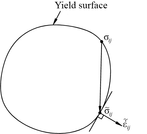
From the associated flow rule, a variational principle can be developed as follows. Let \(\tilde{v}_i\) be a kinematically admissible velocity field. This velocity field must satisfy the essential boundary conditions and the incompressibility condition. Let \(\sigma_{ij}\) and \(\tilde{\sigma}_{ij}\) be the actual stress and the stress corresponding to the admissible velocity field \(\tilde{v}_i\), respectively. As shown in Figure 4.2, from the convexity of the yield surface and the normality of the strain rate, the following relationship always holds.

\[ \sum_{i=1}^{3} \sum_{j=1}^{3} (\tilde{\sigma}_{ij} - \sigma_{ij}) \dot{\tilde{\varepsilon}}_{ij} \ge 0 \tag{4.40} \]

Here, the equality holds only when \(\tilde{\sigma}_{ij} = \sigma_{ij}\). Meanwhile, since

\[ \begin{aligned} \sum_i \sum_j \int_V \sigma_{ij} \dot{\tilde{\varepsilon}}_{ij} dV &= \sum_i \sum_j \int_V \sigma_{ij} \frac{\partial \tilde{v}_i}{\partial x_j} dV \\ &= \sum_i \sum_j \left[ \int_{S_{t_i}} \bar{t}_i \tilde{v}_i dS + \int_{S_{v_i}} \sigma_{ij} n_j \bar{v}_i dS - \int_V \frac{\partial \sigma_{ij}}{\partial x_j} \tilde{v}_i dV \right] \\ &= \sum_i \sum_j \left[ \int_{S_{t_i}} \bar{t}_i \tilde{v}_i dS + \int_{S_{v_i}} \sigma_{ij} n_j \bar{v}_i dS \right] \end{aligned} \tag{4.41} \]

substituting this relationship into Eq. (4.40) yields the following inequality.

\[ \sum_i \sum_j \int_V \tilde{\sigma}_{ij} \dot{\tilde{\varepsilon}}_{ij} dV - \sum_i \int_{S_{t_i}} \bar{t}_i \tilde{v}_i dS \ge \sum_i \sum_j \int_{S_{v_i}} \sigma_{ij} n_j \bar{v}_i dS \tag{4.42} \]

In the above equation, the equality holds when \(\tilde{\sigma}_{ij} = \sigma_{ij}\). That is, when the admissible velocity field coincides with the exact solution, the functional on the left-hand side attains its minimum value. Therefore, this problem is formulated as an extremization problem of the functional, i.e. as a variational principle. Meanwhile, if the material obeys the von Mises yield theory and has isotropic hardening properties, then since

\[ \sum_i \sum_j \tilde{\sigma}_{ij} \dot{\tilde{\varepsilon}}_{ij} = \tilde{\bar{\sigma}} \dot{\tilde{\bar{\varepsilon}}} \tag{4.43} \]

the following functional is obtained.

\[ \phi = \int_V \tilde{\bar{\sigma}} \dot{\tilde{\bar{\varepsilon}}} dV - \sum_i \int_{S_{t_i}} \bar{t}_i \tilde{v}_i dS \tag{4.44} \]

That is, the admissible velocity field \(\tilde{v}_i\) that minimizes Eq. (4.44) is the solution sought.

Figure 4.2 Relationship between stress and strain rate

4.4 Flow stress

The factors affecting the analysis results are the initial conditions of the material, the flow stress, friction, velocity, etc., and these are the essential information about the target process that an engineer must possess. Empirically, among these, the influence of the flow stress is the greatest. The plastic deformation characteristics of a material, i.e. the flow stress, are affected by various variables. Elastic strain, plastic strain, anisotropy, strain rate, temperature, recrystallization and grain size, damage, etc. are examples of variables that affect the plastic deformation characteristics of a material. The influence of these variables on the flow stress, i.e. the functional relationship between the flow stress and the variables, is complex, and the degree of influence changes sensitively with temperature.

Figure 4.3 Influence of temperature, strain, and strain rate on flow stress

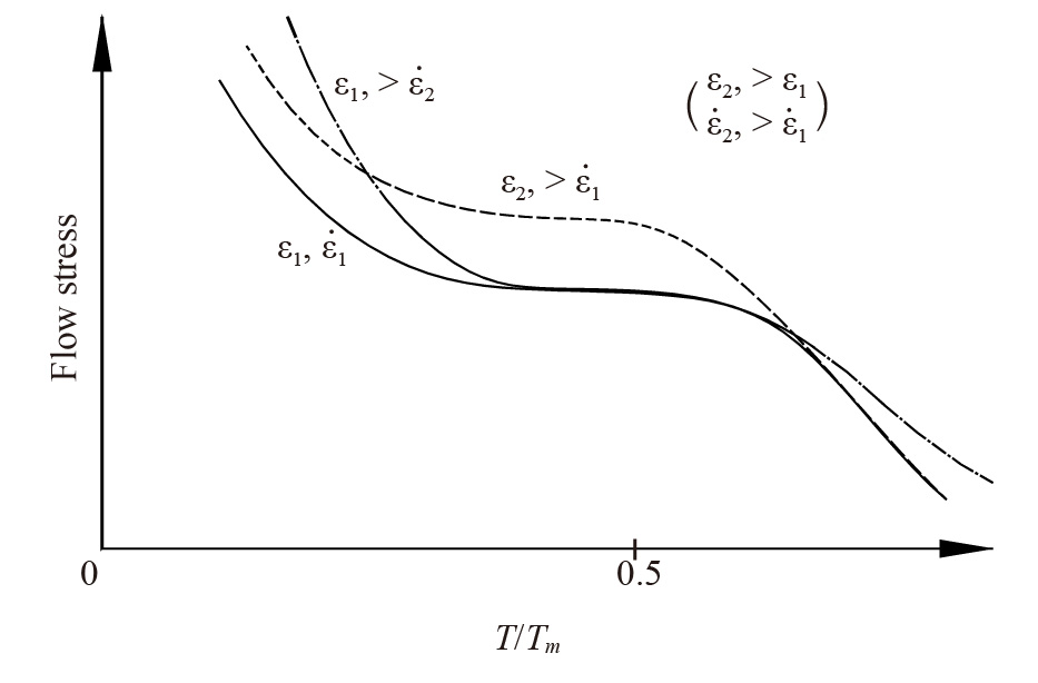
Figure 4.3 illustrates the influence of temperature, strain, strain rate, etc. on the flow stress function of a material. In the figure, \(T_m\) denotes the melting-point temperature of the material. At low temperatures, strain and strain rate have a relatively large influence on the flow stress function, and it can be seen that as the temperature approaches room temperature the influence of strain rate diminishes. From room temperature up to just before the recrystallization temperature, the influence of strain is large while the influence of strain rate is negligibly small, whereas above the recrystallization temperature the influence of strain diminishes. Thus, plasticity problems are generally solved under the assumption that materials are strain-dependent at room temperature and strain-rate-dependent at high temperatures.

Figure 4.4 shows the influence of strain on the flow stress function. At high temperatures, when the strain reaches a critical value, recrystallization occurs, so the change in the flow stress function with increasing strain is slight. At low temperatures, the strain dependence of industrial materials is relatively high. Figure 4.5 shows the influence of strain rate on the flow stress function at high temperatures. The flow stress function is composed of roughly three regions. If the strain rate is below a certain value or above a certain value, the flow stress increases with increasing strain rate. In the intermediate region, the change in flow stress with increasing strain rate is not large. General metal forming is carried out in the intermediate region and the left region, and in ultra-high-speed forming such as explosive forming, the strain rate can belong to the right region.

Figure 4.4 Strain and flow stress

Figure 4.5 Influence of strain rate on flow stress at high temperature

There is no change in the mechanical laws just because the material is different. Only the material coefficients associated with the constitutive equation change. The yield stress \(\bar{\sigma}\) of a material undergoing plastic deformation is a function of the effective strain \(\bar{\varepsilon}\), the effective strain rate \(\dot{\bar{\varepsilon}}\), the temperature \(T\), the damage \(D\), the grain size \(G\), the microstructure \(M\), etc., and reflects the mechanical properties or state of the material. This function is called the flow stress.

A material whose flow stress does not depend on strain or strain rate, i.e. a material with constant flow stress, is called a perfectly plastic material, and a material whose flow stress is a function of the plastic strain \(\bar{\varepsilon}^p\) only, i.e.

\[ \bar{\sigma} = \bar{\sigma}(\bar{\varepsilon}^p) \tag{4.45} \]

is called a rigid-plastic material. The flow stresses of viscoplastic and thermoviscoplastic materials are expressed respectively by the following equations.

\[ \bar{\sigma} = \bar{\sigma}(\bar{\varepsilon}^p, \dot{\bar{\varepsilon}}^p) \tag{4.46} \]

\[ \bar{\sigma} = \bar{\sigma}(\bar{\varepsilon}^p, \dot{\bar{\varepsilon}}^p, T) \tag{4.47} \]

In the case of a thermoviscoplastic material, temperature affects the stress, so temperature analysis and flow analysis must be carried out simultaneously. Such an analysis is called a non-isothermal analysis or a coupled analysis. If the temperature during the process is assumed to be constant, it becomes a viscoplastic flow stress, and the analysis under these process conditions is called an isothermal analysis.