2 Stress

2.1 Definition of Stress

In engineering, force itself is important, but the force acting per unit area, that is, stress, is essential for the development and application of theory. The physical meaning of stress is the force acting per unit area, and its dimension is [force][length]\(^{-2}\). Since stress generally differs at each material point, it is a function of the position of the material point, that is, of the coordinates \(x_i\) or (\(x_1\), \(x_2\), \(x_3\)). Although a vector in three-dimensional space has three components, stress is expressed by nine components, of which the number of independent stress components is six.

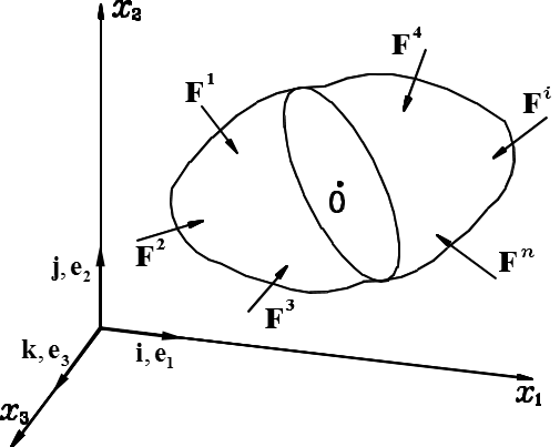
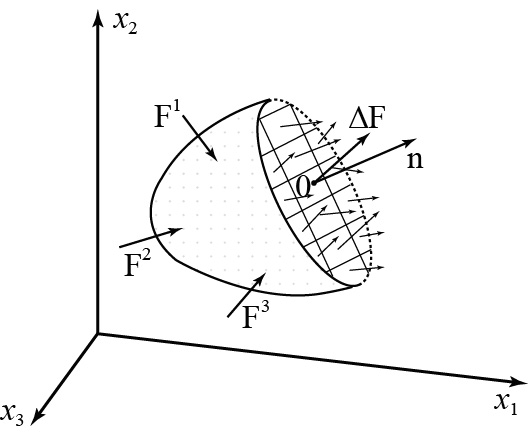
Before the mathematical definition of stress, let us study the stress vector. In Figure 2.1, consider a hypothetical cut passing through an arbitrary point \(O\) inside or on the boundary of the object of interest. On this cut, as shown in Figure 2.2, internal forces that follow the law of action and reaction act in the form of a distributed load in order to maintain force balance. As shown in the figure, let the outwardly directed unit normal vector of the cut be \(\mathbf{n}\) or \(n_i\), and let the resultant of the internal forces acting on the cross-sectional area \(\Delta A\) centered at point \(O\) be \(\Delta F\). Then, the stress vector at point \(O\) with respect to \(\mathbf{n}\) is defined as follows.

\[ t^{(n)}=\lim_{\Delta A \to 0 } \frac{\Delta F}{\Delta A} \tag{2.1} \]

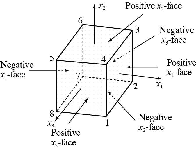
Since the stress vector is defined at a point of the object, it is a function of position. In the definition of the stress vector in Eq. (2.1), the outwardly directed unit normal vector \(\mathbf{n}\) and \(\Delta A \to 0\) must be kept in mind. That is, although a point has neither area nor volume, in order to define the stress vector at a point, the direction and magnitude of the area of interest are taken into account. Figure 2.3 defines faces in order to explain stress or the stress vector. If the outward normal vector of a face coincides with the \(x_1\)-axis, it is defined as the positive \(x_1\)-face, and if it points in the direction opposite to the \(x_1\)-axis, it is called the negative \(x_1\)-face. The \(x_2\)-face and \(x_3\)-face are defined in the same way. Although area itself can never inherently be negative, since a cut passing through a point always forms a pair of two faces, the positive face and the negative face are defined for the purpose of distinguishing those faces.

Figure 2.1 Object of interest and loads

Figure 2.2 Internal force acting on the face whose outwardly directed unit normal vector is

Figure 2.3 Definition of the positive face and the negative face

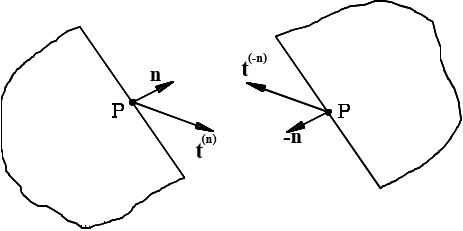
On the other hand, as shown in Figure 2.4, when the object is separated at an arbitrary point \(P\), two faces are created, and these two faces are defined by the outward normal vectors \(\mathbf{n}\) and -\(\mathbf{n}\). On the separated faces, the forces per unit area acting at point \(P\), that is, \(t^{(n)}\) and \(t^{(-n)}\), must be equal in magnitude and opposite in direction by Newton's third law of motion, that is, the law of action and reaction. That is,

\[\mathbf{t}^{(n)} = -\mathbf{t}^{(-n)} \quad \text{or} \quad t_i^{(n)} = -t_i^{(-n)} \tag{2.2}\]

holds.

Figure 2.4 The law of action and reaction

When the vector \(\mathbf{n}\) coincides with the \(x_1\)-axis, that is, when \(\mathbf{n=i}\) or \(e_1\), the \(x_1, x_2, x_3\)-components of the stress vector \(\mathbf{t}^{(\mathbf{n})}\) are defined as \(\sigma_{11}, \sigma_{12}, \sigma_{13}\) (or \(\sigma_{xx}, \sigma_{xy}, \sigma_{xz}\)), respectively. That is,

\[\mathbf{t}^{(\mathbf{e}_1)} = \sum_{i=1}^{3} \sigma_{1i} \mathbf{e}_i \quad \text{or} \quad t_j^{(\mathbf{e}_1)} = \sigma_{1j} = \lim_{\Delta A_1 \to 0} \frac{\Delta F_j}{\Delta A_1} \tag{2.3}\]

holds. Here, \(\Delta A_1\) denotes the infinitesimal area on the \(x_1\)-face on which the resultant \(\Delta \mathbf{F}\) is defined, and \(\mathbf{e}_i\) is the unit vector of the \(x_i\)-axis, as shown in Figure 2.1. In the same way, the stress components \(\sigma_{21}, \sigma_{22}, \sigma_{23}, \sigma_{31}, \sigma_{32}, \sigma_{33}\), etc., are defined. That is, generalizing Eq. (2.3) yields the following.

\[t_j^{(\mathbf{e}_i)} \equiv \sigma_{ij} = \lim_{\Delta A_i \to 0} \frac{\Delta F_j}{\Delta A_i} \tag{2.4}\]

Here, \(A_i\) is the infinitesimal area on the area defined by \(\mathbf{n} = \mathbf{e}_i\). Therefore, the stress \(\sigma_{ij}\) denotes the force per unit area in the \(j\) direction acting on the \(i\) face. The components \(\sigma_{11}, \sigma_{22}, \sigma_{33}\), whose subscripts \(i\) and \(j\) are identical, are normal stresses, and the components \(\sigma_{12}, \sigma_{23}, \sigma_{31}, \sigma_{21}, \sigma_{32}, \sigma_{13}\), etc., whose subscripts differ, are shear stresses. Shear stresses are often expressed using \(\tau\) instead of \(\sigma\), and normal stresses are expressed using a single subscript. For example, \(\sigma_{12} (\sigma_{xy})\) is sometimes expressed as \(\tau_{12} (\tau_{xy})\), and a normal stress \(\sigma_{11} (\sigma_{xx})\) is sometimes expressed as \(\sigma_x\). Since a normal stress is the case in which the force acts perpendicular to the face, it represents a tensile (positive) or compressive (negative) stress. Since a shear stress acts in a direction parallel to the area, it has the meaning of shear force per unit area. Expressing the stress components in matrix form gives the following.

\[\begin{bmatrix} \sigma_{11} & \sigma_{12} & \sigma_{13} \\ \sigma_{21} & \sigma_{22} & \sigma_{23} \\ \sigma_{31} & \sigma_{32} & \sigma_{33} \end{bmatrix} \quad \text{or} \quad \begin{bmatrix} \sigma_{xx} & \sigma_{xy} & \sigma_{xz} \\ \sigma_{yx} & \sigma_{yy} & \sigma_{yz} \\ \sigma_{zx} & \sigma_{zy} & \sigma_{zz} \end{bmatrix} \tag{2.5}\]

Let us consider the sign of stress. Hypothetical cuts passing through a point of a solid form pairs of two. As described above, if one of them is called the \(\mathbf{n}\) face (positive face), the other will be the \(-\mathbf{n}\) face (negative face). By the law of action and reaction in Eq. (2.2), forces equal in magnitude and opposite in direction act on the positive face and the negative face. Therefore, the fact that the stress components acting at the same point on the two hypothetical cuts created by a single cut are identical can be seen from the following equation.

\[t_j^{(\mathbf{e}_i)} = -t_j^{(-\mathbf{e}_i)} \equiv \sigma_{ij} \tag{2.6}\]

From this equation, the (+) sign of a stress component means that a load in the positive direction acts on the positive face or a load in the negative direction acts on the negative face, and otherwise it becomes a stress with the (-) sign. Therefore, a positive normal stress component means that a tensile stress acts in the direction of that component.

Let us reconsider the process of expressing the stress at a point. A coordinate system is needed to express the shape of an object numerically. The coordinate system can be chosen conveniently according to the problem. Since in the numerical analysis (finite element analysis, etc.) of solid mechanics problems the solution of virtually all problems is possible using only the rectangular (or Cartesian) coordinate system, from now on the rectangular coordinate system is mainly explained. Of course, if an axisymmetric problem is formulated in a cylindrical coordinate system, a two-dimensional approach can be applied, so the cylindrical coordinate system is mainly used. The orientation of the rectangular coordinate system may be chosen conveniently. In general, the widely used \(x-y\) coordinate system consisting of horizontal and vertical lines is pleasing to the eye and effective in terms of space utilization. However, from the viewpoint of mechanics, it can be effective to use a rectangular coordinate system with a special orientation. For example, using a coordinate system that coincides with the principal stress axes is advantageous from the viewpoint of the development of theory and grasping physical meaning. The specific content of this is detailed in Section 2.3.

Stress is a second-order tensor quantity [1.1]. Therefore, the stress tensor of the same point with respect to different coordinate systems follows the following coordinate transformation law.

\[\sigma_{i'j'} = \sum_{p=1}^{3} \sum_{q=1}^{3} T_{i'p} T_{j'q} \sigma_{pq}\]

or

\[\begin{pmatrix} \sigma_{1'1'} & \sigma_{1'2'} & \sigma_{1'3'} \\ \sigma_{2'1'} & \sigma_{2'2'} & \sigma_{2'3'} \\ \sigma_{3'1'} & \sigma_{3'2'} & \sigma_{3'3'} \end{pmatrix} = \begin{pmatrix} T_{1'1} & T_{1'2} & T_{1'3} \\ T_{2'1} & T_{2'2} & T_{2'3} \\ T_{3'1} & T_{3'2} & T_{3'3} \end{pmatrix} \begin{pmatrix} \sigma_{11} & \sigma_{12} & \sigma_{13} \\ \sigma_{21} & \sigma_{22} & \sigma_{23} \\ \sigma_{31} & \sigma_{32} & \sigma_{33} \end{pmatrix} \begin{pmatrix} T_{1'1} & T_{2'1} & T_{3'1} \\ T_{1'2} & T_{2'2} & T_{3'2} \\ T_{1'3} & T_{2'3} & T_{3'3} \end{pmatrix} \tag{2.7}\]

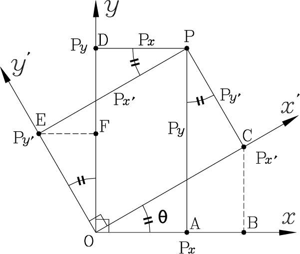
Here, \(T_{i'p}\) is a component of the transformation matrix, and is the cosine value of the angle between the \(x_{i'}\)-axis and the \(x_p\)-axis. That is,

\[T_{i'p} = \cos(x_{i'}, x_p) \tag{2.8}\]

holds.

Among stress tensors, when the components with respect to one axis (usually regarded as the \(x_3\)-axis (or \(z\)-axis)) are all zero, this stress is called plane stress. Problems such as rectangular-section beams and thin plates are representative examples of plane stress. For plane stress, the transformation relationship between the two coordinate systems in Figure 2.5 is as follows.

\[\begin{bmatrix} \sigma_{1'1'} & \sigma_{1'2'} \\ \sigma_{2'1'} & \sigma_{2'2'} \end{bmatrix} = \begin{bmatrix} \cos\theta & \sin\theta \\ -\sin\theta & \cos\theta \end{bmatrix} \begin{bmatrix} \sigma_{11} & \sigma_{12} \\ \sigma_{21} & \sigma_{22} \end{bmatrix} \begin{bmatrix} \cos\theta & -\sin\theta \\ \sin\theta & \cos\theta \end{bmatrix} \tag{2.9}\]

What must be emphasized here is the fact that, even though their numerical values differ, the two sets of stress components in Eq. (2.9) have the same physical meaning. In particular, since Eq. (2.9) is a similarity transformation, the eigenvalues of the two stress tensors, that is, the principal stresses, are identical. Of course, this point also holds in three-dimensional space in the same way.

Figure 2.5 Coordinate transformation

On the other hand, the stress vector \(\mathbf{t}^{(n)}\) and the stress tensor \(\sigma_{ij}\) are in the following relationship.

\[t_i^{(n)} = \sum_{j=1}^{3} \sigma_{ji} n_j \quad \text{or}\]

\[\begin{bmatrix} t_x^{(n)} \\ t_y^{(n)} \\ t_z^{(n)} \end{bmatrix} = \begin{bmatrix} \sigma_{xx} & \sigma_{xy} & \sigma_{xz} \\ \sigma_{yx} & \sigma_{yy} & \sigma_{yz} \\ \sigma_{zx} & \sigma_{zy} & \sigma_{zz} \end{bmatrix} \begin{bmatrix} n_x \\ n_y \\ n_z \end{bmatrix} \tag{2.10}\]

This relation is called Cauchy's formula. From this formula, if the stress at a point is known, the stress vector for an arbitrary direction, that is, the force acting per unit area, can be obtained, and on a boundary \(S_t\) where the surface traction vector is given as \(t_i^{(n)} = \bar{t}_i\), the boundary condition can be expressed in terms of stress components. That is,

\[\sum_{j=1}^{3} \sigma_{ji} n_j = \bar{t}_i \quad \text{on} \quad S_t \tag{2.11}\]

holds. In this equation, the right-hand side is a known value, and on the left-hand side the vector \(n_j\) is the outward unit normal vector defined at the boundary, which is a known value determined geometrically at the boundary; therefore, a boundary on which the surface traction vector is given is a boundary on which a condition regarding stress is given.

2.2 Equilibrium Equations

If the effect of acceleration can be neglected, then from the equilibrium conditions the sum of all external forces must be zero, and the sum of the first moments of the external forces must also be zero. And this condition must hold also for an arbitrary volume \(V'\) virtually separated from the solid of interest in Figure 2.6. Of course, when the equilibrium condition is applied to the separated volume \(V'\), the internal forces that were acting on the boundary \(S'\) before separation must be regarded as external forces acting on \(S'\), which is the boundary of the separated volume \(V'\).

Figure 2.6 Solid and subsystem

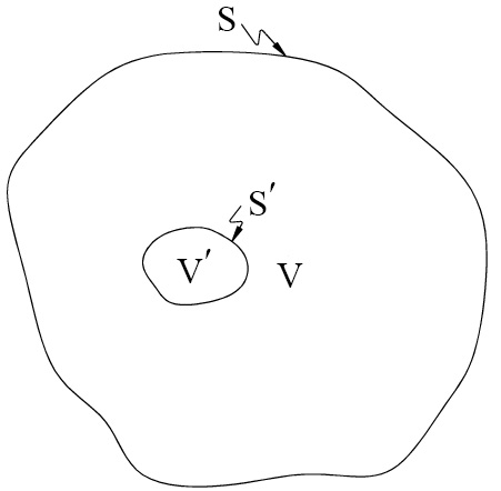
External forces include body forces and surface tractions, and since from the equilibrium condition the sum of the external forces must be zero,

\[\int_{S'} t_i^{(n)} dS + \int_{V'} f_i dV = 0 \quad (i=1,2,3) \tag{2.12}\]

holds. Here, \(f_i\) denotes the body force per unit volume. Using Cauchy's formula of Eq. (2.10) and the divergence theorem, Eq. (2.12) becomes

\[\int_{V'} \left( \sum_{j=1}^{3} \frac{\partial \sigma_{ji}}{\partial x_j} + f_i \right) dV = 0 \tag{2.13}\]

and since this equation must hold for an arbitrary subsystem \(V'\),

\[\sum_{j=1}^{3} \frac{\partial \sigma_{ji}}{\partial x_j} + f_i = 0 \quad \text{or} \quad \begin{matrix} \frac{\partial \sigma_{xx}}{\partial x} + \frac{\partial \sigma_{yx}}{\partial y} + \frac{\partial \sigma_{zx}}{\partial z} + f_x = 0 \\ \frac{\partial \sigma_{xy}}{\partial x} + \frac{\partial \sigma_{yy}}{\partial y} + \frac{\partial \sigma_{zy}}{\partial z} + f_y = 0 \\ \frac{\partial \sigma_{xz}}{\partial x} + \frac{\partial \sigma_{yz}}{\partial y} + \frac{\partial \sigma_{zz}}{\partial z} + f_z = 0 \end{matrix} \tag{2.14}\]

must hold. This equation is called the equation of equilibrium. In elasticity and plasticity, the equilibrium equation of Eq. (2.14) is taken as the governing equation. If the effect of acceleration cannot be neglected, the following equation of motion corresponding to the equilibrium equation is derived.

\[\sum_{j=1}^{3} \frac{\partial \sigma_{ji}}{\partial x_j} + f_i = \rho \dot{v}_i \tag{2.15}\]

Here, \(\dot{v}_i\) is the acceleration. In Eqs. (2.14) and (2.15), the first term is called the diffusion term. In solid mechanics, the convective term, which reflects the acceleration term arising from the flow of the material, is neglected. On the other hand, from the condition that the sum of the moments for the subsystem must be zero,

\[\int_{S'} \mathbf{x} \times \mathbf{t}^{(n)} dS + \int_{V'} \mathbf{x} \times \mathbf{f} dV = \mathbf{0}\]

or

\[\sum_{j=1}^{3} \sum_{k=1}^{3} \int_{S'} \varepsilon_{ijk} x_j t_k^{(n)} dS + \sum_{j=1}^{3} \sum_{k=1}^{3} \int_{V'} \varepsilon_{ijk} x_j f_k dV = 0 \quad (i=1, 2, 3) \tag{2.16}\]

holds. Here, \(\varepsilon_{ijk}\) is the permutation symbol, and is defined as follows according to the indices \(i\), \(j\), \(k\).

\[\varepsilon_{ijk} = \begin{cases} 0 & \text{if } i=j \text{ or } k=i \\ 1 & \text{if } (i, j, k) = (1, 2, 3) \text{ or } (2, 3, 1) \text{ or } (3, 1, 2) \\ -1 & \text{if } (i, j, k) = (1, 3, 2) \text{ or } (2, 1, 3) \text{ or } (3, 2, 1) \end{cases} \tag{2.17}\]

From Cauchy's formula and the divergence theorem,

\[\sum_{j=1}^{3} \sum_{k=1}^{3} \int_{V'} \varepsilon_{ijk} \left[ x_j \left( \sum_{p=1}^{3} \frac{\partial \sigma_{pk}}{\partial x_p} + f_k \right) + \sigma_{jk} \right] dV = 0 \quad (i=1,2,3) \tag{2.18}\]

is obtained.

From the equilibrium equation, since \(\sum_{p=1}^{3} \partial \sigma_{pk} / \partial x_p + f_k = 0\),

\[\sum_{j=1}^{3} \sum_{k=1}^{3} \varepsilon_{ijk} \sigma_{jk} = 0 \quad (i=1,2,3) \tag{2.19}\]

holds. Therefore, since \(\varepsilon_{ijk}\) is skew-symmetric with respect to \(j\) and \(k\), \(\sigma_{ij}\) must be symmetric. That is,

\[\sigma_{ij} = \sigma_{ji} \quad \text{or} \quad \sigma_{xy} = \sigma_{yx}, \sigma_{yz} = \sigma_{zy}, \sigma_{zx} = \sigma_{xz} \tag{2.20}\]

holds. Eqs. (2.14) and (2.20) establish the interrelationships among the stress components, and the stress components that satisfy these relations become the stress distribution to be sought in static or quasi-static mechanics problems such as elasticity and plasticity.

2.3 Principal Stresses and Stress Invariants

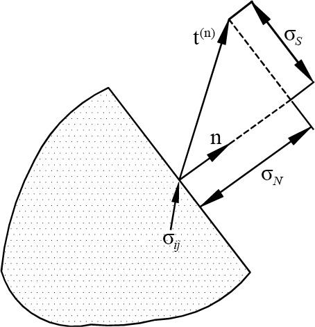
As shown in Figure 2.7, taking the dot product of the stress vector and the outwardly directed unit normal vector gives

\[\sigma_N = \mathbf{t}^{(n)} \cdot \mathbf{n} = \sum_{i=1}^{3} t_i^{(n)} n_i = \sum_{i=1}^{3} \sum_{j=1}^{3} \sigma_{ji} n_i n_j \tag{2.21}\]

and \(\sigma_N\) becomes the normal component of the stress vector, that is, the normal stress component. The direction in which this normal stress component becomes maximum is called the principal stress direction, and its magnitude is called the principal stress. Viewed from the principal stress axis, the stress vector and the outward normal vector lie on the same straight line. That is, \(t_i^{(n)} \propto n_i\). Therefore, the shear stress component on the principal stress axis is zero, and the principal stress direction \(\mathbf{n}\) and the principal stress magnitude \(\sigma_N\) must satisfy the following relationship.

Figure 2.7 Stress vector and its normal and tangential stress components

\[t_i^{(n)} = \sum_{j=1}^{3} \sigma_{ij} n_j = \sigma_N n_i \quad \text{or} \quad \begin{bmatrix} \sigma_{xx} & \sigma_{xy} & \sigma_{xz} \\ \sigma_{yx} & \sigma_{yy} & \sigma_{yz} \\ \sigma_{zx} & \sigma_{zy} & \sigma_{zz} \end{bmatrix} \begin{bmatrix} n_x \\ n_y \\ n_z \end{bmatrix} = \sigma_N \begin{bmatrix} n_x \\ n_y \\ n_z \end{bmatrix} \tag{2.22}\]

Eq. (2.22) is a homogeneous linear equation and an eigenvalue problem. In order for this eigenvalue problem to have a meaningful solution, the following characteristic equation must be satisfied.

\[|\sigma_{ij} - \sigma_N \delta_{ij}| = 0 \quad \text{or} \quad \begin{vmatrix} \sigma_{xx} - \sigma_N & \sigma_{xy} & \sigma_{xz} \\ \sigma_{yx} & \sigma_{yy} - \sigma_N & \sigma_{yz} \\ \sigma_{zx} & \sigma_{zy} & \sigma_{zz} - \sigma_N \end{vmatrix} = 0 \tag{2.23}\]

This characteristic equation carries the meaning of making Eq. (2.22) indeterminate so that it has infinitely many solutions. That is, it makes the linear equations linearly dependent. Organizing this condition derives the following cubic algebraic equation.

\[\sigma_N^3 - I_1 \sigma_N^2 - I_2 \sigma_N - I_3 = 0 \tag{2.24}\]

Here, \(I_1, I_2, I_3\) are defined as follows.

\[I_1 = \sum_{i=1}^{3} \sigma_{ii} = \sigma_{xx} + \sigma_{yy} + \sigma_{zz} \tag{2.25}\]

\[\begin{aligned} I_2 &= \frac{1}{2} \sum_{i=1}^{3} \sum_{j=1}^{3} (\sigma_{ij}\sigma_{ij} - \sigma_{ii}\sigma_{jj}) \\ &= -\sigma_{xx}\sigma_{yy} - \sigma_{yy}\sigma_{zz} - \sigma_{zz}\sigma_{xx} + \sigma_{xy}^2 + \sigma_{yz}^2 + \sigma_{zx}^2 \end{aligned} \tag{2.26}\]

\[I_3 = |\sigma_{ij}| = \sigma_{xx}\sigma_{yy}\sigma_{zz} + 2\sigma_{xy}\sigma_{yz}\sigma_{zx} - \sigma_{xx}\sigma_{yz}^2 - \sigma_{yy}\sigma_{zx}^2 - \sigma_{zz}\sigma_{xy}^2 \tag{2.27}\]

Since the stress tensor is symmetric, by the theory of linear algebra Eq. (2.24) has three real roots \(\sigma_1, \sigma_2, \sigma_3\) (generally ordered as \(\sigma_1 \ge \sigma_2 \ge \sigma_3\)). \(\sigma_1, \sigma_2, \sigma_3\) have the physical meaning of principal stresses and are the eigenvalues of the stress tensor. Among the principal stresses, the maximum and minimum values become the maximum and minimum normal stresses, respectively. The direction of the vector \(\mathbf{n}^{(i)}\) obtained by substituting each principal stress \(\sigma_i\) into \(\sigma_N\) of Eq. (2.22) becomes the direction of the principal stress axis corresponding to the principal stress \(\sigma_i\). It is noteworthy that the shear stress with respect to the principal stress axes is zero. And since the three principal stress axes \(\mathbf{n}^{(i)}\) can be regarded as mutually orthogonal, the following relationship holds.

\[\mathbf{n}^{(i)} \cdot \mathbf{n}^{(j)} = \delta_{ij} \tag{2.28}\]

Here, \(\delta_{ij}\) is the Kronecker delta, which has the value 1 if \(i\) and \(j\) are identical and 0 if they differ. The principal stresses (eigenvalues) are values independent of the coordinate system, since stress is a second-order tensor quantity. That is, if the stress state at a point is given, the magnitudes and directions of the principal stresses are already determined. The coordinate system merely provides a reference for expressing or quantifying position and mechanical quantities. Therefore, in Eq. (2.24), \(I_1, I_2, I_3\) are values determined independently of the coordinate system, and are the stress invariants. Therefore, if the stress invariants of Eqs. (2.25)–(2.27) are expressed with respect to the principal stress axes, since the shear stresses on the principal stress axes are zero,

\[I_1 = \sigma_1 + \sigma_2 + \sigma_3 \tag{2.29}\]

\[I_2 = -\sigma_1\sigma_2 - \sigma_2\sigma_3 - \sigma_3\sigma_1 \tag{2.30}\]

\[I_3 = \sigma_1\sigma_2\sigma_3 \tag{2.31}\]

are simplified, and \(I_1, I_2, I_3\) are called the first stress invariant, the second stress invariant, and the third stress invariant, respectively. As seen in Eqs. (2.29)–(2.31), the principal stress axes allow the stress invariants to be expressed concisely and facilitate the development of theory.

2.4 Deviatoric Stress Tensor and Effective Stress

\(\sigma_m = I_1 / 3\) is the mean stress, and the negative of the mean stress, that is, \(p = -\sigma_m\), is called the hydrostatic pressure. In general, it has been found that hydrostatic pressure does not significantly affect the plastic deformation of a material. Therefore, the deviatoric stress tensor obtained by subtracting the mean stress from the normal components of the stress tensor,

\[\sigma_{ij}' = \sigma_{ij} - \sum_{k=1}^{3} \frac{\sigma_{kk}}{3} \delta_{ij} \tag{2.32}\]

is frequently used for the purpose of developing theory. Here, \(\delta_{ij}\) is the Kronecker delta. The deviatoric stress tensor \(\sigma_{ij}'\) is a second-order tensor quantity and has the following three invariants.

\[J_1 = 0 \tag{2.33}\]

\[J_2 = \frac{1}{2} \sum_{i=1}^{3} \sum_{j=1}^{3} \sigma_{ij}' \sigma_{ij}' = \frac{1}{2} ({\sigma_1'}^2 + {\sigma_2'}^2 + {\sigma_3'}^2) \tag{2.34}\]

\[J_3 = |\sigma_{ij}'| = \sigma_1' \sigma_2' \sigma_3' \tag{2.35}\]

Therefore, since the first invariant of the deviatoric stress tensor is always zero, the invariants of the deviatoric tensor are in effect two. On the other hand, separating the effect of \(I_1\) from \(I_2\), \(I_2\) is organized as follows.

\[\begin{aligned} I_2 &= -\frac{1}{3}I_1^2 + \frac{1}{6}[(\sigma_{xx} - \sigma_{yy})^2 + (\sigma_{yy} - \sigma_{zz})^2 + (\sigma_{zz} - \sigma_{xx})^2 + 6\sigma_{xy}^2 + 6\sigma_{yz}^2 + 6\sigma_{zx}^2] \\ &= -\frac{1}{3}I_1^2 + \frac{1}{6}[(\sigma_1 - \sigma_2)^2 + (\sigma_2 - \sigma_3)^2 + (\sigma_3 - \sigma_1)^2] \\ &= -\frac{1}{3}I_1^2 + \frac{1}{2} \sum_{i=1}^{3} \sum_{j=1}^{3} \sigma_{ij}' \sigma_{ij}' \\ &= -\frac{1}{3}I_1^2 + J_2 \end{aligned} \tag{2.36}\]

Therefore, it can be seen that \(J_2\) is \(I_2\) with the effect of the hydrostatic pressure (\(I_1\)) excluded. The effective stress or equivalent stress \(\bar{\sigma}\) is defined as follows.

\[\begin{aligned} \bar{\sigma} &= \sqrt{3J_2} \\ &= \sqrt{\frac{3}{2} \sum_{i=1}^{3} \sum_{j=1}^{3} \sigma_{ij}' \sigma_{ij}'} \\ &= \sqrt{\frac{1}{2} [(\sigma_{xx} - \sigma_{yy})^2 + (\sigma_{yy} - \sigma_{zz})^2 + (\sigma_{zz} - \sigma_{xx})^2 + 6\sigma_{xy}^2 + 6\sigma_{yz}^2 + 6\sigma_{zx}^2]} \\ &= \sqrt{\frac{1}{2} [(\sigma_1 - \sigma_2)^2 + (\sigma_2 - \sigma_3)^2 + (\sigma_3 - \sigma_1)^2]} \end{aligned} \tag{2.37}\]

The effective stress expresses a three-dimensional or two-dimensional stress as a value corresponding to the stress in a simple tension test.

2.5 Two-Dimensional Mechanics Problems and Axisymmetric Problems

Two-dimensional solid mechanics problems are formulated as plane stress problems and plane strain problems, and axisymmetric problems are also classified as two-dimensional problems. In a strict sense, most actual two-dimensional problems belong to three-dimensional problems, but they are defined under the assumption of a two-dimensional plane stress or plane strain problem. This is because, in engineering, obtaining three-dimensional analysis results requires much effort and cost, and it is not easy to directly utilize three-dimensional analysis results for the purpose of problem solving.

Figure 2.8 Plane stress

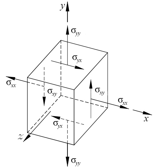
As shown in Figure 2.8, when the stress components for a certain single direction in three-dimensional space are all zero, this stress is called plane stress. In general, the \(z(x_3)\)-direction is made to coincide with the direction in which the stress components are zero. Therefore, the stress of a plane stress problem is expressed by the following equation.

\[\begin{bmatrix} \sigma_{11} & \sigma_{12} \\ \sigma_{21} & \sigma_{22} \end{bmatrix} \quad \text{or} \quad \begin{bmatrix} \sigma_{xx} & \sigma_{xy} \\ \sigma_{yx} & \sigma_{yy} \end{bmatrix} \tag{2.38}\]

On the other hand, a solid mechanics problem in which the load conditions, material properties, boundary conditions, etc., are all axisymmetric is called an axisymmetric problem. To be axisymmetric, the plane formed by the axis and every line segment passing through the center of a cross section perpendicular to the axis must be a plane of symmetry. An axisymmetric problem is actually a three-dimensional problem, but analysis on a two-dimensional plane is possible. This is because the mechanical behavior on all planes of symmetry is identical. In the process of formulating an axisymmetric problem as an analysis problem on a two-dimensional plane, no assumptions or approximations are involved. However, some of the coefficients inherent in the actual three-dimensional differential equations expressed in the cylindrical coordinate system are transformed into functions of the coordinates in the corresponding two-dimensional differential equations.

(a) Three-dimensional problem (b) Axisymmetric problem

Figure 2.9 Stress tensor in the cylindrical coordinate system and the axisymmetric problem

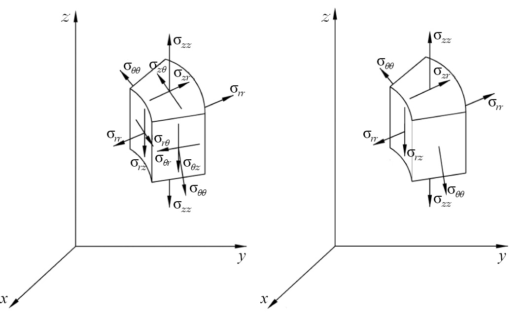
Axisymmetric problems are formulated in the \(r-\theta-z\) cylindrical coordinate system. Figure 2.9(a) defines the stress tensor \(\sigma_{ij}\) in the cylindrical coordinate system. That is,

\[\begin{bmatrix} \sigma_{rr} & \sigma_{r\theta} & \sigma_{rz} \\ \sigma_{\theta r} & \sigma_{\theta\theta} & \sigma_{\theta z} \\ \sigma_{zr} & \sigma_{z\theta} & \sigma_{zz} \end{bmatrix} \tag{2.39}\]

holds. From symmetry arguments, for an axisymmetric problem

\[\sigma_{r\theta} = \sigma_{\theta z} = 0 \tag{2.40}\]

so the stress components of an axisymmetric problem are as shown in Figure 2.9(b). That is, the non-zero stress components in an axisymmetric problem are as follows.

\[\begin{bmatrix} \sigma_{rr} & 0 & \sigma_{rz} \\ 0 & \sigma_{\theta\theta} & 0 \\ \sigma_{zr} & 0 & \sigma_{zz} \end{bmatrix} \tag{2.41}\]

2.6 Isotropic Yield Theory

When the effect of self-weight is not considered, if no force is applied to a solid, all stress components are zero and no deformation occurs. If a load below a certain magnitude is applied and then removed, the solid returns to its original shape. The deformation in this case is called elastic deformation. If a force above a certain magnitude is applied and then removed, part of the deformation is elastically recovered and the rest remains in the object as permanent deformation; this is called plastic deformation.

Sand or manganese nodules existing at a depth of 10000 m under the sea are under the influence of a very large hydrostatic pressure \(p\) of about 1000 atm. On this object, normal stresses whose absolute values are very large compared with the yield strength of the material, that is, \(\sigma_x = \sigma_y = \sigma_z = -p\), act. If this stress state caused fracture or plastic deformation, the sea would become deeper and deeper, and ultimately the Earth would collapse. The fact that the Earth is not collapsing tells us that merely large stress components do not cause plastic deformation or fracture. The question is: at what stress state does a material begin to undergo plastic deformation? Strictly speaking, there is no exact answer to this question. There are only hypotheses and theories, that is, yield theories, and the validity of a yield theory differs slightly from material to material.

First, let us study the deformation behavior of a material under uniaxial tension in Figure 2.10(a). Figure 2.10(b) shows the stress state and the true stress \(\sigma_t\)–true strain \(\varepsilon_t\) curve in a uniaxial tension test. In this problem, stresses other than \(\sigma_{11} = \sigma_t\) are zero. In a state with no residual stress, when \(\sigma_{11}\) is increased from 0 and reaches the initial yield stress \(Y_o\) (\(\sigma_{11} = Y_o\)), initial plastic deformation occurs. In general, when plastic deformation occurs, most metallic materials exhibit the ability to resist additional deformation, that is, the property of strain hardening. As shown in Figure 2.10(b), with the increase of strain, the yield stress at that instant, that is, the flow stress \(Y\), increases. For most metallic materials, if the force is removed after causing plastic deformation, elastic recovery occurs along line \(BC\), which is parallel to line \(OA\) in Figure 2.10(b). If the force is applied again, it is assumed to reach the yield point \(B\) along \(CB\). Of course, in reality there may be a slight difference, but in most cases the difference is negligible. Therefore, in a certain state, that is, at \(\varepsilon = \varepsilon_t\), if the stress \(\sigma_{11}\) is less than the flow stress \(Y(\varepsilon_t)\), that is, if \(\sigma_{11} \le Y(\varepsilon_t)\), the object remains in an elastic state. But can \(\sigma_{11} > Y(\varepsilon_t)\) occur? At point B, \(\sigma_{11} > Y_o\), but for a material that has already undergone plastic deformation and become strain-hardened, \(Y_o\) is meaningless. \(\sigma_{11} > Y(\varepsilon_t)\) can never occur.

(a) Tension test

(b) True stress-true strain curve

Figure 2.10 Tension test and the true stress-true strain curve

In order to evaluate the stress state and quantify plastic deformation, a yield function \(f\) is defined. The yield function is a function of stress, that is,

\[f = f(\sigma_{ij}) \tag{2.42}\]

and it is a function whose meaning is that if the function value \(f\) for the stress at a certain point is negative, that point exists in the elastic region, and if the function value is 0, it belongs to the plastic region. However, the yield function cannot be positive. That is,

\[\begin{aligned} &f(\sigma_{ij}) < 0 : \sigma_{ij}\text{ exists within the elastic region.} \\ &f(\sigma_{ij}) = 0 : \sigma_{ij}\text{ exists on the yield surface.} \\ &f(\sigma_{ij}) > 0 : \text{is impossible.} \end{aligned} \tag{2.43}\]

holds. In the tension test described above, the yield function is \(f = \sigma_{11} - Y\).

Drucker's postulate plays an important role in the development of the theory of plasticity. That is, Drucker's postulate leads to the results that the yield surface (curved surface) must be convex and that the strain rate tensor corresponding to a point on the yield surface must be perpendicular to the yield surface. This is called the associated flow rule. Drucker's postulate is summarized as follows.

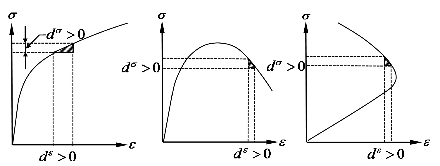
① In the process of applying a load, the added stress must do positive work. ② When an additional stress is applied and then removed, if plastic deformation has occurred, the total work done must be positive. And if the deformation of a strain-hardening material took place within the elastic range, the work done must be zero. ③ As a result, the shape of the true stress–true strain curve must be as in Figure 2.11(a), and Figures 2.11(b) and 2.11(c) violate Drucker's postulate. ④ Drucker's postulate yields the results that the yield surface must be convex and that the plastic strain rate occurs in the direction perpendicular to the yield surface.

Figure 2.11 Drucker's postulate

A stress of a certain state that causes yielding can be expressed with different component values depending on the coordinate system, but fundamentally the yielding phenomenon itself cannot be avoided. That is, although the stress tensor is expressed with different values depending on direction, the yielding phenomenon, which is directly connected to the magnitude of the stress, is independent of the coordinate system used to define the stress. Therefore, it can be expected that there is a deep correlation between the stress invariants and the yielding phenomenon. If a material has isotropic hardening, since yielding must be independent of the coordinate system, the yield function \(f\) must be a function of the stress invariants \(I_1, I_2, I_3\). That is, the yield function must have the following form.

\[f(I_1, I_2, I_3) = 0 \tag{2.44}\]

In general, unless it is a porous material, a material does not undergo fracture or plastic deformation under a hydrostatic pressure state of appropriate magnitude. Therefore, the effect of \(I_1\) on the yielding of the material is neglected. The yield function in this case must be

\[f(J_2, J_3) = 0 \tag{2.45}\]

Here, \(J_2\) and \(J_3\) are the invariants of the deviatoric stress, and are defined by the following equations.

\[J_2 = \frac{1}{2} \sum_{i=1}^{3} \sum_{j=1}^{3} \sigma_{ij}' \sigma_{ij}' = \frac{1}{2} ({\sigma_1'}^2 + {\sigma_2'}^2 + {\sigma_3'}^2) = -\frac{1}{3} I_1^2 + I_2 \tag{2.46}\]

\[J_3 = |\sigma_{ij}'| = \sigma_1' \sigma_2' \sigma_3' \tag{2.47}\]

From this equation, it can be seen that with respect to \(\sigma_i'\), \(J_2\) is an even function and \(J_3\) is an odd function. If yielding occurred when the stress state of an isotropic material was \((\sigma_1', \sigma_2', \sigma_3')\), yielding must also occur when it is \((-\sigma_1', \sigma_2', \sigma_3')\). However, since \(J_3(\sigma_1', \sigma_2', \sigma_3') = -J_3(-\sigma_1', \sigma_2', \sigma_3')\), the yield function \(f\) must be an even function with respect to \(J_3\). For instance, it must be included in the yield function as terms such as the square or the fourth power of \(J_3\). Therefore, it is not highly realistic.

The strain-hardening phenomenon of a material is explained by isotropic hardening and kinematic hardening. Isotropic hardening is a term referring to an ideal hardening characteristic based on the assumption that even if a material has been hardened by compressive deformation, it exhibits the same hardening capacity when tensile deformation is applied. That is, isotropic hardening is a hardening characteristic based on the assumption that if compressive deformation is applied to a tensile specimen of a material so that the yield stress increases from \(Y_1\) to \(Y_2\), and then a tensile force is applied, initial yielding occurs when a tensile stress of \(Y_2\) acts. It can be said that, in a strict sense, there is no material exhibiting such a characteristic. However, since the change of deformation mode during plastic forming is not extreme, and when it is extreme there is a process of relaxing the degree of strain hardening through heat treatment, empirically the assumption of isotropic hardening does not produce a large error. However, the Bauschinger effect and the like cannot be expressed by isotropic hardening.

Above, we have studied the basic requirements that a yield function must have. A number of yield criteria that are widely used while satisfying these requirements have been introduced. The von Mises (or Huber-von Mises) yield criterion and the Tresca yield criterion are representative yield criteria.

2.6.1 von Mises Yield Criterion

The von Mises yield criterion is the most widely used theory among yield criteria for the purpose of analyzing plastic forming processes. This is because the associated flow rule is expressed in a clear closed-form mathematical expression and its superiority has also been proven experimentally. The von Mises yield criterion is the theory that a material yields when the stress state satisfies the following equation.

\[f = J_2 - k^2 = \frac{1}{2} \sum_{i=1}^{3} \sum_{j=1}^{3} \sigma_{ij}' \sigma_{ij}' - k^2 = 0\]

or

\[\bar{\sigma} = \sqrt{\frac{1}{2} [(\sigma_{xx} - \sigma_{yy})^2 + (\sigma_{yy} - \sigma_{zz})^2 + (\sigma_{zz} - \sigma_{xx})^2] + 3\sigma_{xy}^2 + 3\sigma_{yz}^2 + 3\sigma_{zx}^2} = Y \tag{2.48}\]

Here, \(\bar{\sigma}\) is the effective stress or equivalent stress. \(Y\) and \(k\) are the yield stress and the yield stress in pure shear of the material, respectively. Since in a pure torsion test the principal stresses are \(\sigma_1 = k, \sigma_2 = 0, \sigma_3 = -k\) when the pure shear yield stress acting on the material in the yielded state is \(k\), from Eq. (2.48), \(k\) and \(Y\) satisfy the following relationship.

\[k = \frac{Y}{\sqrt{3}} \tag{2.49}\]

The yield stress \(Y\) is a value related to the properties of the material, and is a function of strain, strain rate, temperature, the damage of the material, the microstructure of the material, etc. Therefore, the von Mises yield criterion is the theory that yielding or plastic deformation occurs when the effective stress reaches the yield stress of the material. The fact that this theory reflects actual phenomena well is supported by numerous experimental research results and application experience.

2.6.2 Tresca Yield Criterion

The Tresca yield criterion (maximum shear stress yield criterion) is also widely used. The Tresca yield criterion is formulated as follows.

\[f = \tau_{\max} - k = 0 \tag{2.50}\]

That is, it means that yielding occurs when the maximum shear stress reaches the allowable shear stress \(k\) of the material. In a tension test, at the moment yielding occurs, the maximum principal stress \(\sigma_1\) is \(Y\) and the minimum principal stress \(\sigma_3\) is 0. Therefore, since in a tension test the maximum shear stress \(\tau_{\max}\) when yielding is reached is

\[\tau_{\max} = \frac{\sigma_{\max} - \sigma_{\min}}{2} = \frac{Y}{2} \tag{2.51}\]

the allowable shear stress \(k\) of the material and the yield stress \(Y\) are in the relationship

\[k = \frac{Y}{2} \tag{2.52}\]

The Tresca yield criterion is widely used for hand calculations and approximate analysis for purposes such as strength analysis, but it is rarely used for the purpose of simulating plastic forming processes.

2.6.3 Yield Function for Plane Stress Problems

In plane stress, the direction perpendicular to the plane is always one of the principal stress axes, and the magnitude of the principal stress for that direction is zero. Therefore, for convenience, let \(\sigma_3 = 0\).

Figure 2.12 Yield function and yield locus for plane stress problems

(1) von Mises yield function

Substituting \(J_2 = \frac{1}{6} [(\sigma_1 - \sigma_2)^2 + (\sigma_2 - \sigma_3)^2 + (\sigma_3 - \sigma_1)^2]\) and \(\sigma_3 = 0\) into Eq. (2.48) and organizing, the von Mises yield condition in a plane stress problem is summarized as follows.

\[f = \sigma_1^2 - \sigma_1\sigma_2 + \sigma_2^2 - Y^2 = 0 \tag{2.53}\]

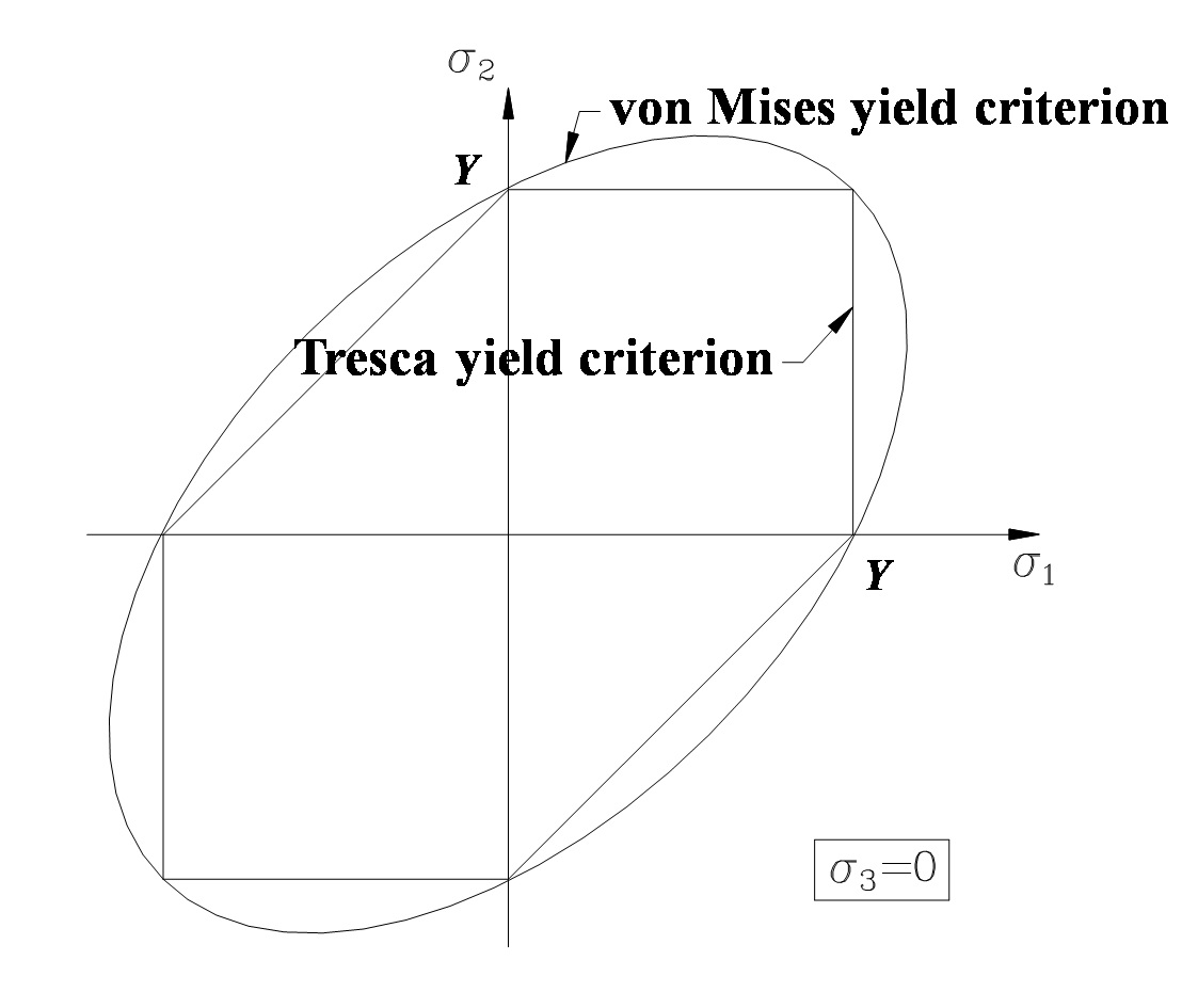
This yield locus is an ellipse, as shown in Figure 2.12, and is convex.

(2) Tresca yield function

The Tresca yield function is expressed as different functions in six regions, as follows.

1. When \(\sigma_1 > \sigma_2 > 0\): \(\tau_{\max} = \sigma_1 / 2 = k = Y / 2, \quad f = \sigma_1 - Y\)
2. When \(\sigma_2 > \sigma_1 > 0\): \(\tau_{\max} = \sigma_2 / 2 = k = Y / 2, \quad f = \sigma_2 - Y\)
3. When \(\sigma_2 > 0 > \sigma_1\): \(\tau_{\max} = (\sigma_2 - \sigma_1) / 2 = k = Y / 2, \quad f = \sigma_2 - \sigma_1 - Y\)
4. When \(0 > \sigma_2 > \sigma_1\): \(\tau_{\max} = -\sigma_1 / 2 = k = Y / 2, \quad f = -\sigma_1 - Y \tag{2.54}\)
5. When \(0 > \sigma_1 > \sigma_2\): \(\tau_{\max} = -\sigma_2 / 2 = k = Y / 2, \quad f = -\sigma_2 - Y\)
6. When \(\sigma_1 > 0 > \sigma_2\): \(\tau_{\max} = (\sigma_1 - \sigma_2) / 2 = k = Y / 2, \quad f = \sigma_1 - \sigma_2 - Y\)

Plotting the yield locus for each region gives Figure 2.12. From the figure, it can be seen that the Tresca yield locus is also convex (strictly speaking, not concave; weakly convex). That is, the line segment connecting two points on the locus exists inside the yield locus or on the yield locus.

2.6.4 von Mises Yield Function for Three-Dimensional Problems

Since the yielding phenomenon of an isotropic material is independent of the coordinate system, it is desirable to express the yield function in terms of principal stresses. In this case, since the three shear stresses become zero, the yield surface can be expressed in three-dimensional space (principal stress axis space) even for a three-dimensional stress problem (six stress components). However, to express the yield surface in a general coordinate system, six coordinate axes are required, so while visualization of the mathematical concept is possible, geometric representation is impossible.

First, let us plot the yield surface in the deviatoric principal stress \(\sigma_1' - \sigma_2' - \sigma_3'\) coordinate system. From the von Mises yield criterion, the yield function \(f(\sigma_1', \sigma_2', \sigma_3')\) is

\[f(\sigma_1', \sigma_2', \sigma_3') = \frac{1}{2}(\sigma_1'^2 + \sigma_2'^2 + \sigma_3'^2) - k^2 \tag{2.55}\]

The yield condition \(f(\sigma_1', \sigma_2', \sigma_3') = 0\) is the equation of a sphere, as shown in Figure 2.13(a).

Now let us plot the yield surface in the principal stress \(\sigma_1 - \sigma_2 - \sigma_3\) coordinate system. Since the yield function \(f(\sigma_1, \sigma_2, \sigma_3)\) is as follows,

\[f(\sigma_1, \sigma_2, \sigma_3) = \frac{1}{6}[(\sigma_1 - \sigma_2)^2 + (\sigma_2 - \sigma_3)^2 + (\sigma_3 - \sigma_1)^2] - k^2 \tag{2.56}\]

the yield surface \(f(\sigma_1, \sigma_2, \sigma_3) = 0\) of a three-dimensional mechanics problem is expressed as in Figure 2.13(b). As shown in the figure, the yield surface is a cylinder whose central axis passes through the origin and whose central axis direction is \((1, 1, 1)\). The plane \(\sigma_1 + \sigma_2 + \sigma_3 = 0\) is called the \(\pi\)-plane, and the locus where this plane and the yield surface meet is called the yield locus \(C\). The locus where the plane \(\sigma_3 = 0\) and the yield surface meet is an ellipse, and is identical to the ellipse in Figure 2.12.

(a) σ'₁-σ'₂-σ'₃ coordinate system

(b) σ₁-σ₂-σ₃ coordinate system

Figure 2.13 Three-dimensional yield surface and yield locus

When the stress state of a point belongs to the interior of the yield surface, that point exists in the elastic region, and when the stress state exists on the cylinder, that point exists in the plastic region. However, as described above, it cannot exist outside the yield surface.