16. Simulation of Sheet Metal Forming and Plate Forging Processes
16.1 Characteristics of Sheet Metal Forming
Metal forming is classified into sheet metal forming and bulk metal forming according to the geometric characteristics of the workpiece or blank. In bulk metal forming, as shown in Figure 16.1⒜, the width, length, and height dimensions of the workpiece are similar, and it mainly results in a change in the cross-sectional shape. Forging, which is representative of bulk metal forming methods, produces metal-part blanks by progressively forming complex lumpy-shaped products using basic processes such as upsetting, extrusion, heading, piercing, trimming, and rolling. Since this has already been described in detail through various application cases earlier, this chapter focuses on content related to sheet metal forming.
Sheet metal forming is a technology that produces the outer skins and interior parts of products by imposing plastic deformation on thin sheets, that is, thin plates. Academically it is also called thin-sheet forming, and in the field it is sometimes called press working or sheet metal work. In general, a sheet metal forming process consists of a multi-stage process in which basic processes such as shear, bending, and drawing are performed in sequence. Figure 16.1⒝ is a conceptualization of sheet metal forming.
In sheet metal forming, the minimum thickness of the deformed sheet is a major concern. That is, process design is generally carried out with the aim of achieving a uniform thickness change. This is because tearing or wrinkling caused by thickness changes during sheet metal forming becomes a cause of poor part reliability or appearance defects. And since sheet-metal-formed products are often used as parts for assemblies to be joined with other parts, minimizing the elastic change caused by residual stress after sheet metal forming, that is, springback, is a major concern for the designer.
Plate forging is a forming method that exploits the advantages of both bulk metal forming and sheet metal forming; it is based on sheet metal forming but locally applies the bulk metal forming method to the necessary parts.

⒜ Bulk metal forming

⒝ Sheet metal forming
Figure 16.1 Characteristics of bulk metal forming and sheet metal forming
Traditional plate forging refers to a method in which an appearance product is first made through deep drawing, bending, and the like, and then the thickness of the desired region is changed through forging. In a broad sense, plate forging includes all cases in which plastic deformation is applied to a sheet with the aim of changing its thickness. In plate forging, since ordinary metal sheets are used as the initial workpiece, the material utilization rate can be maximized compared with CNC machining, and for this reason plate forging has the advantage of being able to shorten CNC machining time by up to several tens of times or more. As shown in Figure 16.2, the plate forging process has higher cost competitiveness than CNC machining, and its precision is also superior to that of other processes.
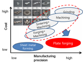
Figure 16.2 Comparison of precision and cost of metal forming
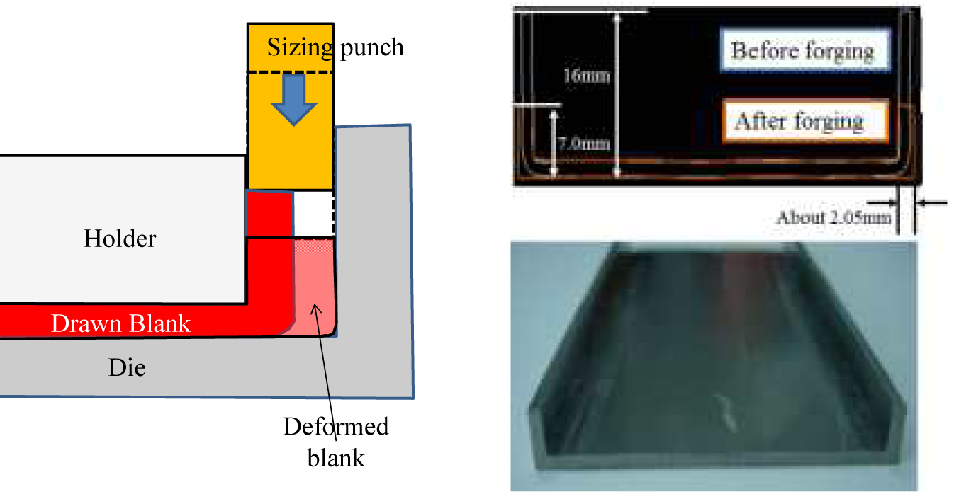
Figure 16.2 Comparison of precision and cost of metal forming
16.2 Classification of Sheet Metal Forming Methods
Among the dies used for the mass production of automotive parts or electronic parts, the press die refers to a mold used to apply an appropriate external pressure to a metal workpiece, thereby inducing plastic deformation in the workpiece to make a product of the desired shape. Sheet metal forming is broadly classified into shearing and forming; the case where the sheet thickness is 6 mm or less is called thin-sheet forming, and the case above that is sometimes called thick-plate forming or plate forging.
This section explains the characteristics of each process and its important design factors rather than the theory of sheet metal forming. The characteristics of the major sheet metal forming operations, excluding the shearing of metal sheets, are summarized below.
(1) Bending process
This refers to the process of bending a sheet using a die. At this time, tensile stress acts on the outer side of the curved surface, and compressive stress acts on the inner side. In the case of the bending process, although the change in shape appears large, the thickness strain is small, and thus the thickness change at the curvature region is also small. The neutral plane of the sheet shifts during the bending process. As plastic deformation ends and elastic recovery takes place, the neutral plane changes owing to the reversal of stress, and an elastic region exists near the neutral plane. After the bending process, the length of the sheet increases. Therefore, an increase in the sheet length occurs owing to the position of the neutral plane of the sheet and the thickness reduction at the curvature region, and its predicted value is utilized in determining the size of the initial blank.
Because the strain remains in the elastic region and the initial plastic region, a springback effect occurs due to elastic recovery after plastic deformation. Since springback causes a large shape change after forming, die design to reduce springback is very important from the standpoint of product assembly.
(2) Deep drawing process
The deep drawing process consists of dies such as a punch, a die, and a blank holder. The sheet placed on the die deforms and is drawn into the interior of the die following the movement of the punch. At this time, a blank holder force is applied to control the drawing speed. The placed sheet is drawn into the die and undergoes a complex stress state of compression (blank holder)-bending (die curvature region)-tension (die wall region). In deep drawing as well, although the change in shape is large, the strain is small. During deep drawing, bending and unbending proceed continuously near the die curvature. At this time, the influence of bending is somewhat large. Therefore, product defects are mainly predicted from the tensile stress or tensile strain of the material.
In the case of cylindrical deep drawing, since the inner diameter within the die is initially smaller than the outer diameter of the blank, wrinkling may occur during forming; to control this, a compressive force is applied with a blank holder, or beads (protrusions) are installed on the die surface at locations where the drawing speed of the material is high, so as to control the speed.
Because the initial blank size affects the success or failure of the process, many initial-blank-size design methods have been proposed. If the initial blank size is excessively large, the sheet tears at the tip of the punch. On the other hand, if the initial blank size is too small, the desired forming height cannot be obtained. In the case of square drawing rather than cylindrical drawing, tearing and wrinkling of the material easily occur owing to the speed difference between the short-side and long-side regions, so optimal initial-blank design becomes very important.
(3) Stretching process
The stretching process is a deformation process in a biaxial tension state, and it is accompanied by a change in thickness. The influence of bending in the stretching process is not as large as in the drawing process, and elastic recovery, that is, springback, is also relatively small. Therefore, it is sometimes applied for springback control. However, in the case of fracture, it may proceed faster than in uniaxial tension.
A typical sheet metal forming process is a process in which bending, drawing, and stretching act in combination, and accurate analysis is possible only when the three effects are considered simultaneously. For accurate finite element analysis, the selection of the material model is important, and in the finite element analysis of sheet metal forming, it is necessary to use elastoplastic continuum elements that consider elasticity and plasticity simultaneously.
16.3 Dies Used in Sheet Metal Forming for Automotive Parts
16.3.1 Blanking Die
A blanking die is a die that cuts or shears steel sheet to produce a blank of dimensions and contour shape suitable for making a product. Figure 16.4 shows a typical blanking die.
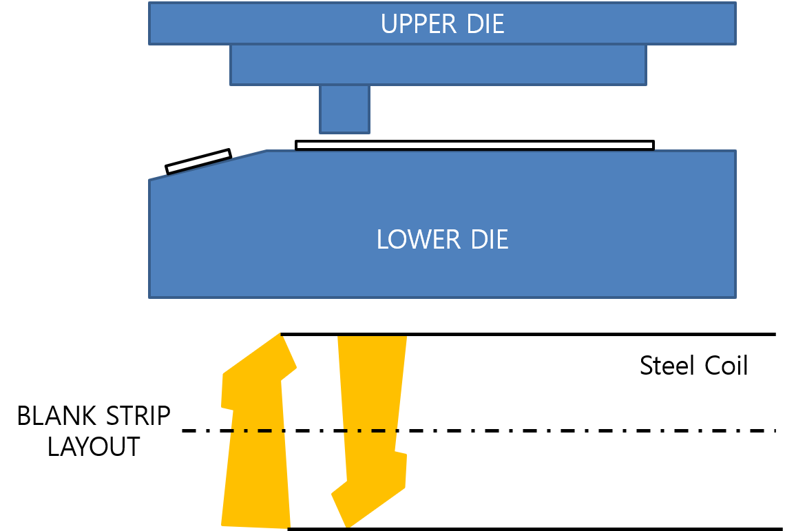
Figure 16.4 Schematic of a blanking die
16.3.2 Drawing Die
A drawing die is a die that forms steel sheet into a bowl-shaped product without the occurrence of wrinkling or fracture. As shown in Figure 16.4, it is classified into single-action or double-action types according to the operating method. The single-action, that is, single-action die, has a structure in which the blank holder on the lower die side is operated by cushion pins, while the double-action or double-action die has a structure in which the punch and blank holder on the upper die side are operated by the outer slide and inner slide of the machine.
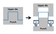
⒜ Single-action drawing
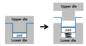
⒝ Double-action drawing
Figure 16.5 Motion diagrams of single-action and double-action dies
16.3.3 Trimming and Piercing Dies
As shown in Figure 16.6, trimming is a die used for the purpose of cutting away and removing the scrap portions of a formed product. Trimming can be performed in various ways according to the shape of the product and the required precision. Piercing is the operation of machining holes inside the blank.

Figure 16.6 Schematic of trimming and piercing
16.3.4 Flanging and Restriking Dies
As shown in Figure 16.6, the operation of cutting off the unnecessary portion of a drawn product and then bending the end of the product to form a flange is called flanging, and the operation of forming a drawn region once more is called restriking.
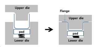
Figure 16.7 Schematic of flanging (top) and restriking (bottom) dies
16.3.5 Cam Die
A press die is a structure that machines the product by up-and-down motion, whereas a cam die is a die that machines by converting the up-and-down motion of the press into horizontal or inclined motion. Figure 16.8 shows a schematic of a typical cam die.
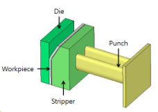
Figure 16.8 Schematic of a cam die
16.4
16.4.1 Analysis Techniques for Thin-Sheet Forming Processes
Approximate solution methods for thin-sheet forming include the slab method, the slip line method, and the upper or lower bound method. These methods each have their own advantages, but in practice most engineering problems are solved by the finite element method. The finite element method is classified in various ways according to the application criterion, as follows.
∙ Geometry: two-dimensional (axisymmetric, plane strain, plane stress) geometry, three-dimensional geometry
∙ Material: elastoplastic material, rigid-plastic material
∙ Magnitude of deformation: large deformation, small deformation
∙ Element characteristics: membrane element, shell/plate element, solid element (or volume element)
∙ Time-based analysis method: implicit approach, explicit approach
16.4.2 Characteristics of Thin-Sheet Forming Analysis
Sheet metal forming is a process of forming a sheet into the required shape by plastic deformation, and unlike bulk metal forming it has the following distinct characteristics. (1) Although the shape change during forming is large, the strain experienced by the material is not large. (2) The changes in sheet thickness and surface area during forming are small. (3) The influence of elastic recovery (springback) is large. (4) The material properties are directional. That is, the influence of anisotropy is large.
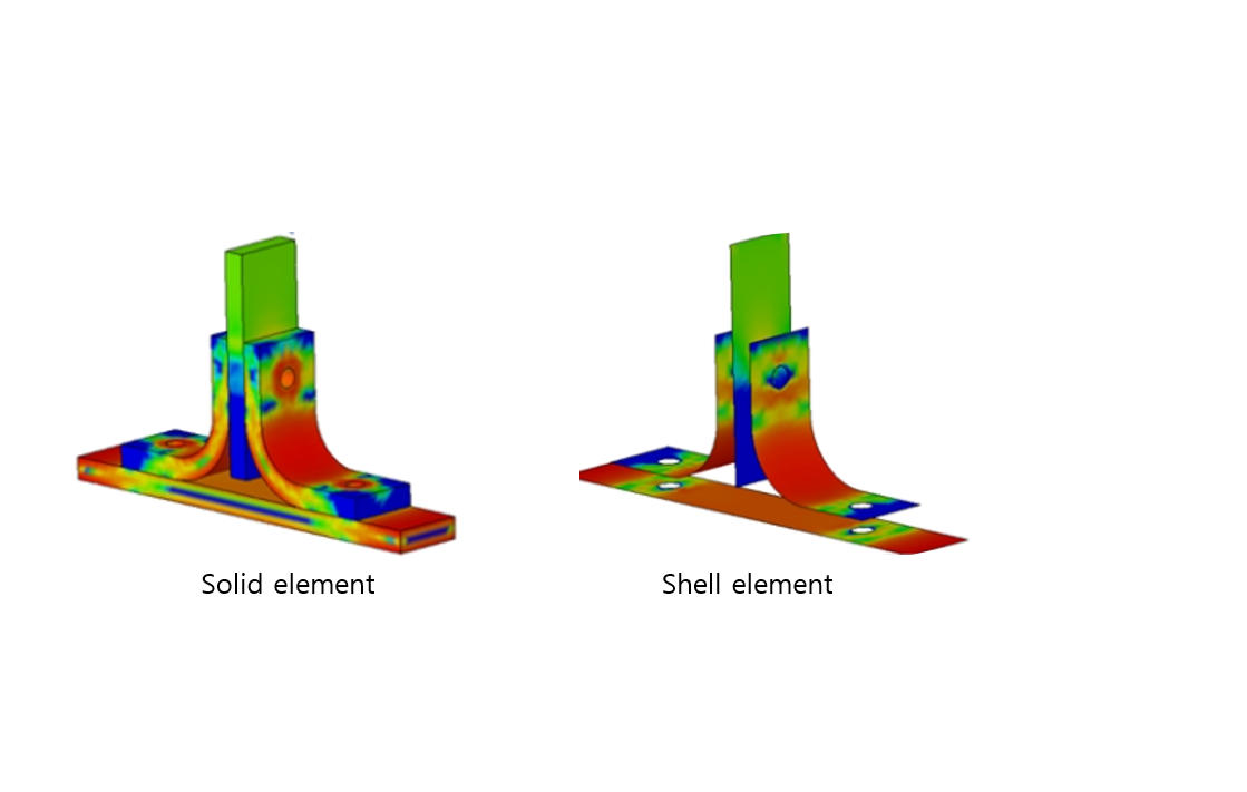
The sheet exhibits anisotropy, having differences in mechanical properties depending on the direction in which stress is applied, owing to the crystallographic directionality of the internal structure that develops through the repeated processes of rolling and annealing during manufacturing. In addition, in the plastic forming of sheets, since the stress acting in the thickness direction is generally relatively small, in most cases a plane stress state of \(\sigma_3 = 0\), with no stress in the thickness direction, is assumed. Therefore, even without using solid elements, using membrane elements or shell/plate elements does not degrade the accuracy of the analysis results while enabling a reduction in analysis time.
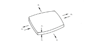
⒜ Stress state of sheet metal forming
⒝ Example of stress analysis
Figure 16.9 Stress states in sheet metal forming and an analysis example
Analysis methods for the sheet metal forming process include the finite element method, the finite difference method, and the upper bound method, and among these the finite element method is the most widely used. In metal sheet metal forming, if the die or process conditions and the like are not properly designed, defects such as fracture, wrinkling, and dimensional inaccuracy occur in the initial part or at an intermediate stage. Since the conventional design of dies and process conditions based on trial and error is burdensome in terms of both cost and required time, process simulation techniques based on the finite element method are being utilized to save cost and time.
The time integration methods used in the finite element method are divided into implicit methods and explicit methods. The implicit method can provide a more accurate solution than the explicit method, and it is known to be efficient for two-dimensional quasi-static problems, for which the contact formulation is relatively simple and the computation is small. On the other hand, in the case of three-dimensional sheet metal forming simulation, the explicit method is more widely applied owing to its simple contact formulation and relatively reasonable level of computation time. The successful use of engineering analysis software for sheet metal forming analysis depends on the efficient generation of shell elements, and in order to accurately predict the final dimensions of sheet-metal-formed parts, springback must fundamentally be taken into account. In the analysis of three-dimensional sheet metal forming processes, the explicit method requires excessive computation time and is therefore not suitable for springback analysis; the general trend is for springback analysis to rely on the implicit method.
The finite element analysis process for sheet metal forming can be broadly divided into three stages: pre-processing, forming analysis, and post-processing. Since this is identical to the analysis of bulk metal forming processes, a detailed explanation is omitted in this section.
The material properties for sheet metal forming process analysis include the yield point, the tensile curve, anisotropy coefficients, friction characteristics, thickness, the forming limit diagram, and the like, and these are mainly obtained by tensile testing. In sheet metal forming analysis, the methods of describing material properties are divided into rigid-plastic and elastoplastic, and different analysis results are predicted depending on the method used to describe the material behavior. Naturally, in sheet metal forming process analysis that emphasizes the thickness change of the sheet caused by stretching, the elastoplastic model is superior to the rigid-plastic model.
Depending on the type of computer time integration method, finite element analysis software is divided into implicit code and explicit code. That is, in order to perform forming analysis, the time-dependent deformation process is calculated through integration, and depending on the method of integration, it is divided into the explicit method and the implicit method. The explicit method calculates \(Y(t+\Delta t)\), the state value after a time increment \(\Delta t\) has elapsed, using the current state value \(Y(t)\), whereas the implicit method obtains \(Y(t+\Delta t)\) through the solution of an equation that includes both \(Y(t+\Delta t)\) and \(Y(t)\). Therefore, the explicit method can have its solution sensitively affected by the time increment \(\Delta t\), whereas the implicit method is relatively robust with respect to the time increment.
The implicit method requires a long computation time and has difficulty with solution convergence, but it is relatively superior in terms of the accuracy of the results. The explicit method can perform analysis in almost all cases, but the accuracy of the analysis results is inferior to that of the implicit method. In most sheet metal forming, shell elements and the explicit method are used; however, in the case of thick plates where the sheet thickness cannot be ignored, in plate forging analysis, or when analysis accuracy is required, the application of the implicit method using solid elements is gradually increasing.
The main features that appear in the formed shape in sheet metal forming include springback, tearing, and wrinkling. The occurrence of shape defects and the like is judged from the strain distribution and formed shape obtained as finite element analysis results, and the adequacy of the shape's dimensional stability due to springback after forming is also judged. By representing the strain state of each region on the forming limit diagram (FLD) of the sheet used for forming, it is possible to evaluate the occurrence of forming defects. The FLD is obtained through dome tests on workpieces of various materials and shapes, and is also calculated by other experimental or theoretical methods.
16.4.3 Application Examples of Sheet Metal Forming Simulation Using Plate Elements
16.4.3.1 Optimal Design of Draw Beads in HSS Steel Sheet Metal Forming
This application example utilizes commercial software dedicated to sheet metal forming process analysis and is a summary of the content contained in Reference [16.3].
Figure 16.10 compares SECC (mild steel) and HSS steel sheet. HSS steel sheet has about 1.5 times the strength of SECC, and its springback will also increase proportionally. Therefore, the application of HSS steel sheet presupposes efficient control of springback.
Figure 16.11 compares the amount of springback obtained using commercial sheet metal forming software in the process of evaluating the two materials from the standpoint of the target process. Shell elements were used, and the explicit method was used.
The red and blue colors represent displacements in opposite directions. Therefore, a feature of the springback in this figure is that a twisting phenomenon occurs. However, although the two materials produce similar twisting, springback and spring-go occur in opposite directions, and the degree of twisting is much greater for HSS. The reason this difference occurs is that the yield strengths differ. Therefore, when forming high-strength steel, applying previously used dies or ordinary die design methods is not appropriate; a die design and process conditions to minimize springback must be presented, and for this the use of simulation technology is essential.
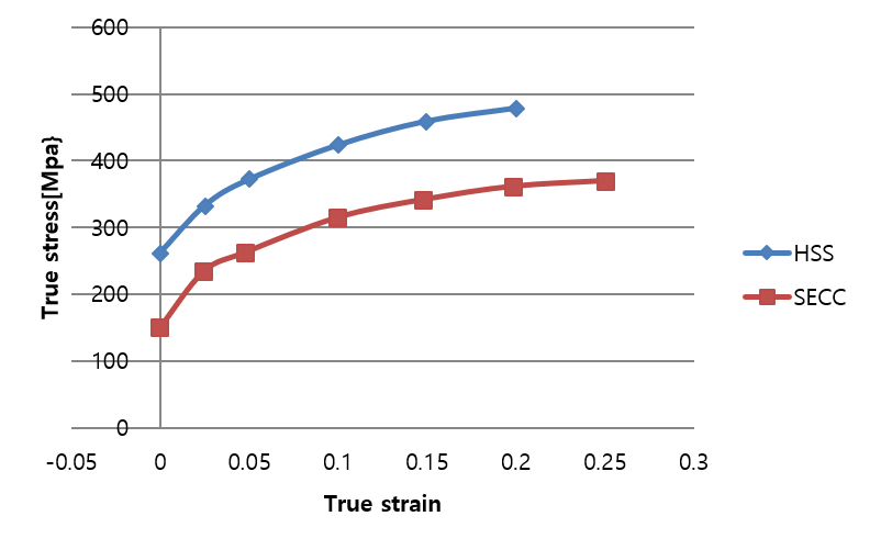
Figure 16.10 Comparison of tensile strength of SECC steel and HSS steel
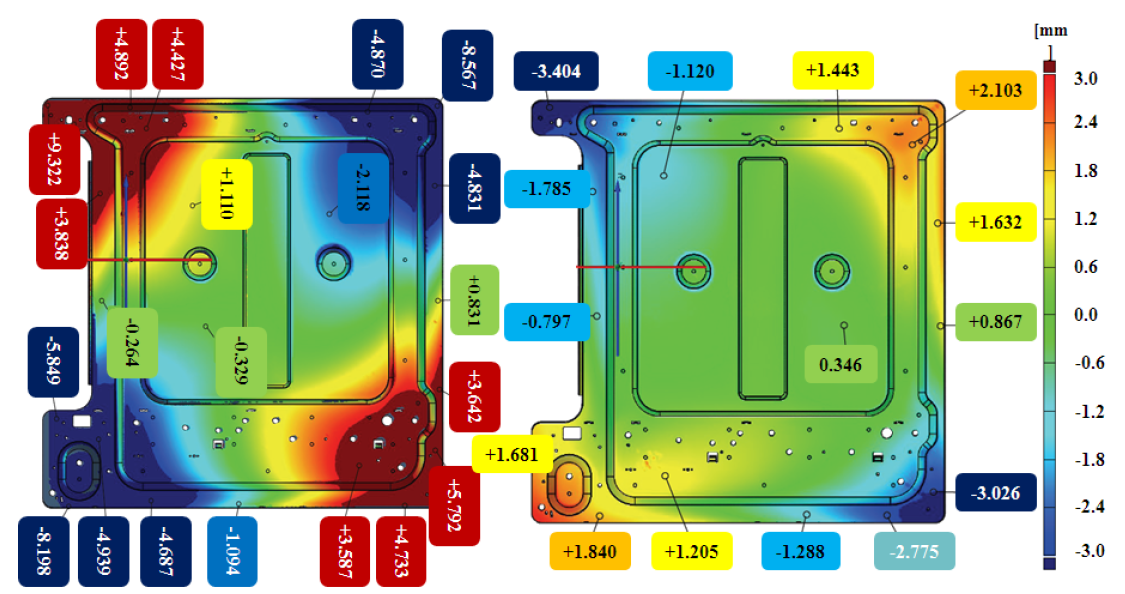
Figure 16.11 Comparison of the degree of springback of HSS steel and SECC steel
Figure 16.12 shows the result of controlling springback by applying tensile force through inducing stretching via engineering optimal design of the draw bead. As shown in this figure, the design that underwent engineering optimization was evaluated as superior in terms of springback compared with the initial design. As a result of performing bead shape optimization through finite element analysis, it was reported that the Z-direction displacement decreased by 37% compared with the previous design and the flatness was very good [16.3].
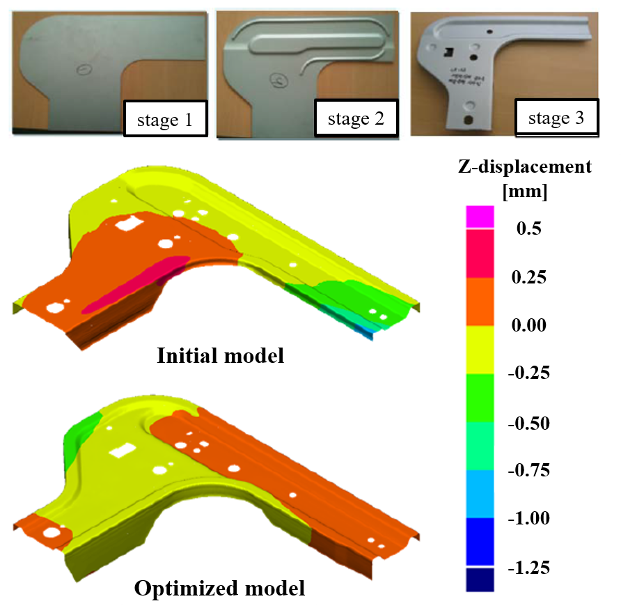
Figure 16.12 Validation of the engineering optimal design of the draw bead
16.4.3.2 Springback Analysis of High-Strength Steel Applying a Kinematic Hardening Model
This application example utilizes commercial software dedicated to sheet metal forming process analysis and is a summary of the content contained in Reference [16.4].
In the case of ordinary steel, since the amount of springback is comparatively small, there is no major problem even if the analysis is performed with an isotropic hardening model without seriously considering the Bauschinger effect. However, high-strength steel is different. In this application example, the influence of the Bauschinger effect on the analysis results of the springback that occurs after forming high-strength steel sheet is analyzed. To account for the Bauschinger effect, the Yoshida-Uemori model was adopted; this model is a two-surface model that assumes the yield surface moves within a bounding surface and is a formulation that expresses both isotropic hardening and kinematic hardening.
Figure 16.13 shows the tension-compression test results for deriving the coefficients of the Yoshida-Uemori kinematic hardening model. In the initial tension region, a work-hardening phenomenon is observed, and along with the typical Bauschinger effect, in which the magnitude of the yield stress in the compression region is slightly lower than the initial tensile yield stress, the elastic slope, that is, the slope of the elastic modulus, also tends to decrease as tension and compression are repeated. These changes in the Bauschinger effect and the elastic slope affect the accuracy of the springback analysis.
Figure 16.14 defines the test process, and Figure 16.15 defines the springback modes and the measured shape dimensions.
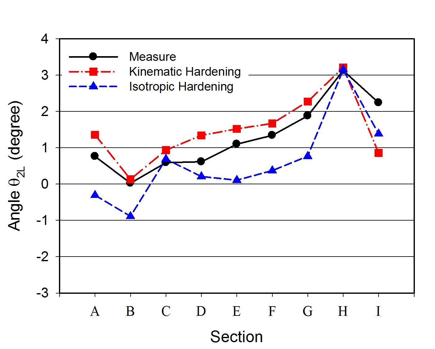
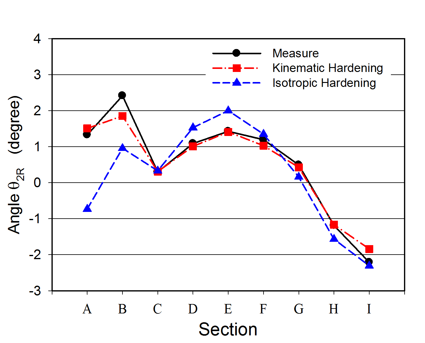
In order to systematically analyze the three-dimensionally occurring springback behavior, the springback occurring in the -direction was investigated at nine cross sections as shown in Figure 16.16. For this purpose, the shape dimensions defined in Figure 16.15 were measured, and the results are shown in Figure 16.17. Figure 16.17 compares the twist angle due to springback and the -direction displacement of the middle region: the experimental results (black, circles), the predicted results of the isotropic hardening model (red, squares), and the predicted results of the kinematic hardening model (blue, triangles). All measurement results indicate that the kinematic hardening model is superior to the isotropic hardening model. That is, overall, the results analyzed with the kinematic hardening model, which can account for the Bauschinger effect, are closer to the actual springback measurement results of the product than the analysis results of the isotropic model.
This example emphasizes the importance of the hardening model in the analysis of the sheet metal forming process of high-strength materials.
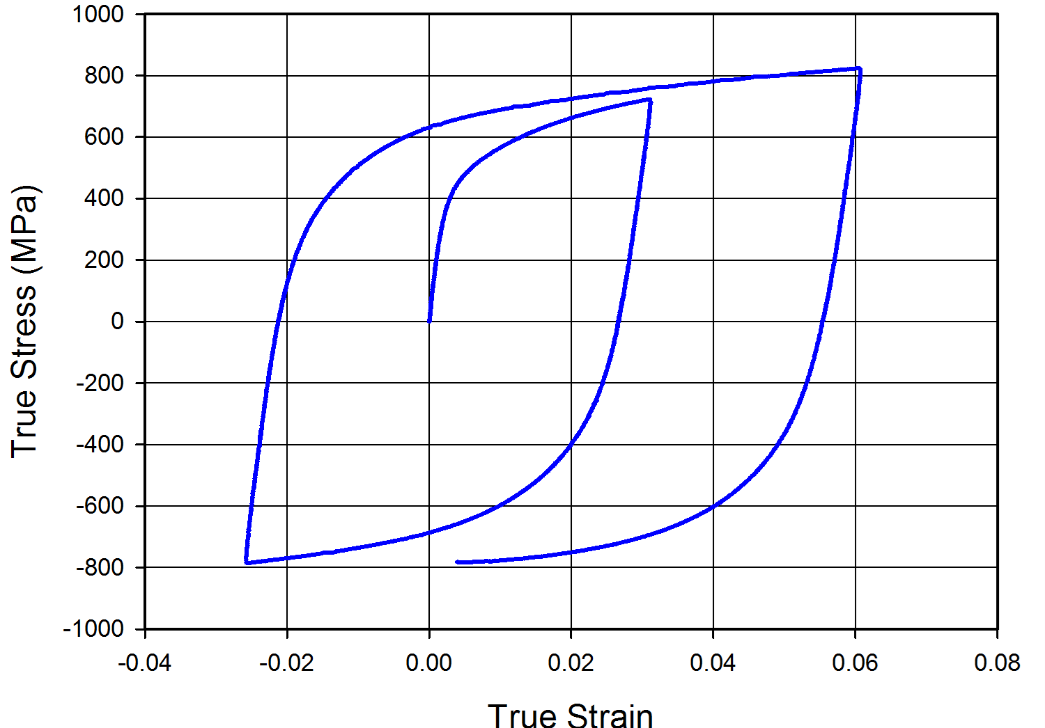
Figure 16.13 Tension-compression test results
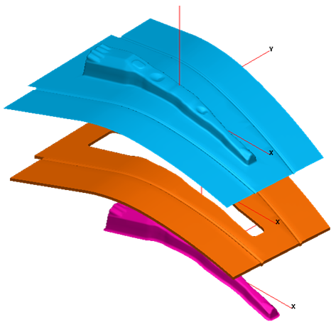
⒜ OP10 Die
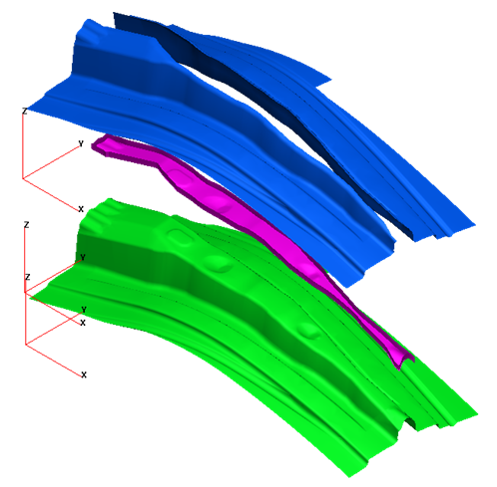
⒝ OP20 Die
Figure 16.14 Reinforce Center Pillar
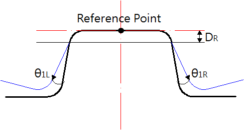
⒜ Wall angle :$\theta_{1L}$, $\theta_{1R}
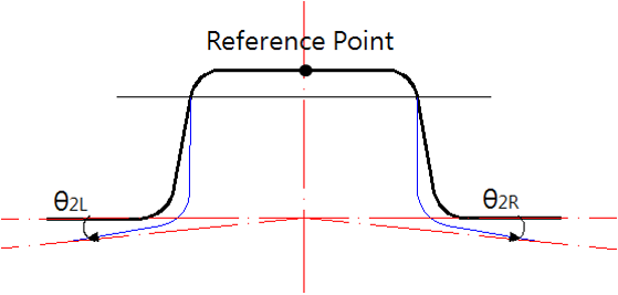
⒝ Flange angle :$\theta_{2L}$, $\theta_{2R}$
Figure 16.15 Springback modes and measured shape dimensions
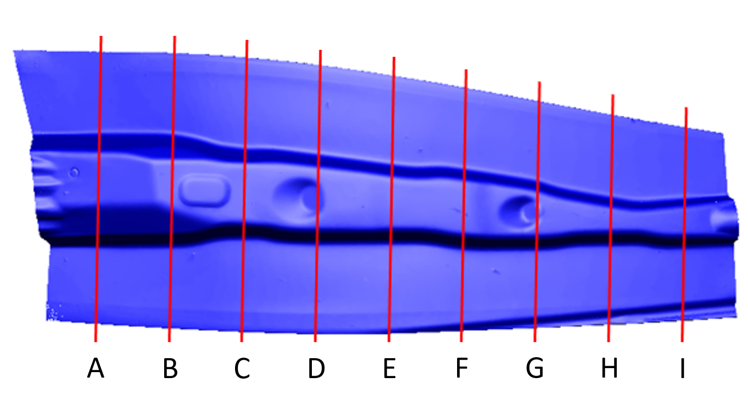
Figure 16.16 Measurement cross sections
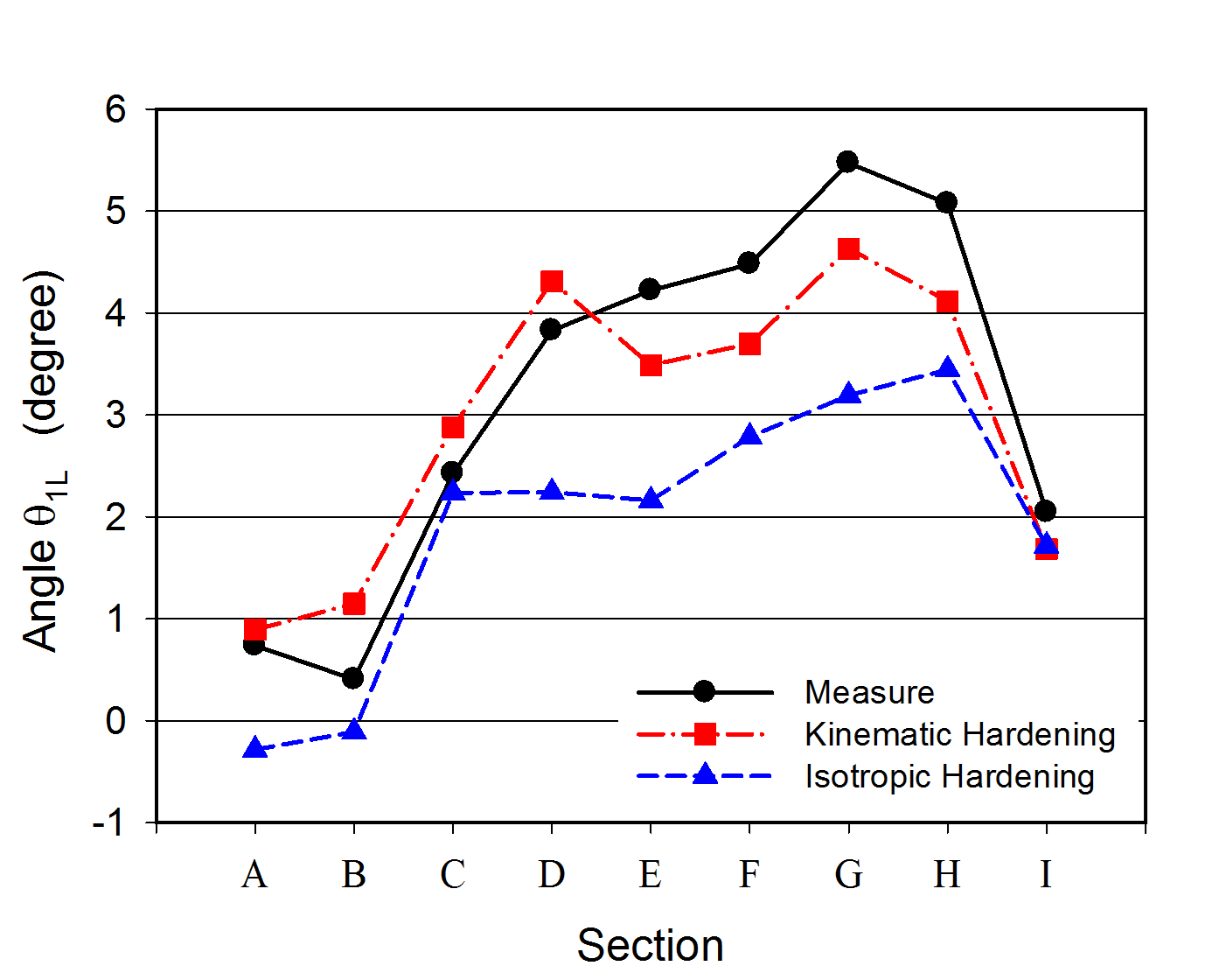
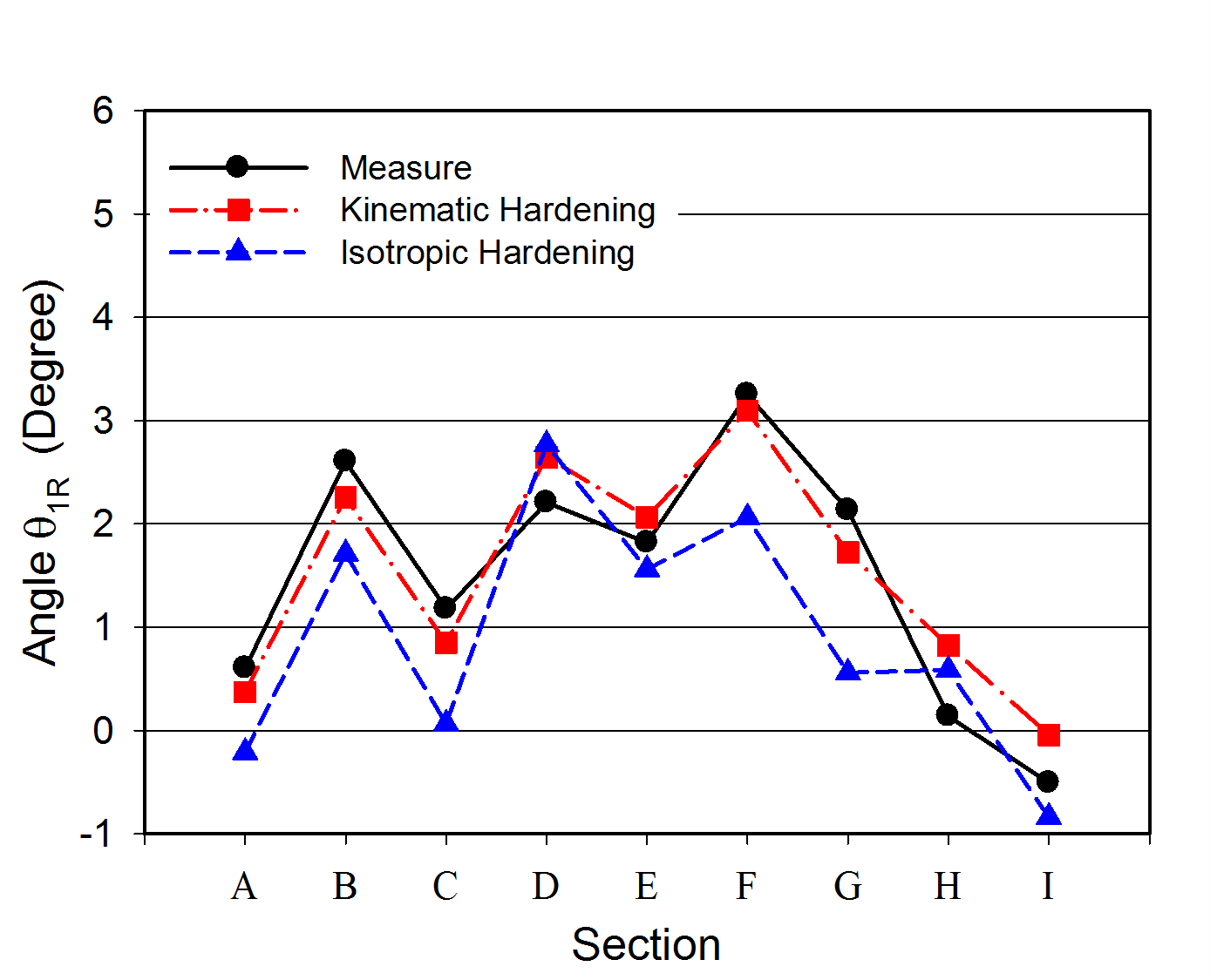
⒜ Wall angle
⒝ Flange angle
Figure 16.17 Comparison of springback after the initial process
16.5 Sheet Metal Forming Analysis Using Volume Elements
16.5.1 Sheet Metal Forming from the Standpoint of Volume Elements
Recent sheet forming analysis programs can consider the elastoplastic properties of materials and provide satisfactory results even for complex die shapes, equipment functions, various changes in forming conditions, continuous processes, and the like. Currently, research on the analysis of innovative sheet forming or plate forging processes, including hydroforming and hot sheet forming processes, is ongoing.
Springback analysis technology provides very valuable information to process design engineers for improving dies and equipment and reducing product errors. However, shell elements, which simplify the numerics and improve computational efficiency, are limited when plastic deformation is applied in the thickness direction. To make matters worse, existing shell elements are very vulnerable when analyzing thick-plate forming or plate forging processes with small corner radii. For this reason, shell elements are not suitable for sheet forming or plate forging process analysis aimed at obtaining precise predictions of plastic deformation in the thickness direction. Currently, plate forging processes devised by forging technology for the purpose of abrupt thickness change are being applied in the automotive and electronics industries for the purpose of simultaneously satisfying structural strength and weight reduction. Therefore, detailed information on plastic deformation at corner regions is bound to be an important subject of interest for process design engineers. As described above, existing sheet forming process analysis techniques are inadequate for satisfying these concerns.
On the other hand, volume elements can be used to improve this problem. In other words, in order to more accurately describe plastic deformation in the thickness direction or near corners, volume elements can be a solution. Various research and applications in this field are being carried out, but they are still at an early stage.
In conclusion, the decisive flaw in the analysis of sheet metal forming processes based on shell elements, membrane elements, plate elements, and the like is that they are unsuitable for processes in which the thickness changes relatively greatly at the corner regions. To solve this problem, the use of volume elements is fundamentally unavoidable. This section introduces analysis techniques and application examples for sheet metal forming processes using volume elements, which have recently been the subject of active application research.
16.5.2 Application Examples of Sheet Metal Forming Simulation Using Volume Elements
16.5.2.1 Analysis of the Square-Cup Deep Drawing Process
Figure 16.18 shows the sheet forming process to be analyzed. It is a square-cup deep drawing process related to an international benchmark conducted at NUMISHEET 93 (square-cup deep drawing process) [16.5]. The workpiece is a square sheet of 150×150×0.78 mm. The flow stress equation of the steel used is \(\bar{\sigma} = 566(0.007 + \bar{\varepsilon})^{0.259}\) MPa, and the yield strength is 167.0 MPa. The binder load is 19.6 kN, and the friction coefficient between the workpiece surfaces is 0.1. Since the punch speed does not affect the solution, it is taken to be 1 mm/s.
The binder load is handled by the binder-load-application technique. That is, the binder is allowed to penetrate the workpiece by a very small, constant distance, and an artificial surface force was imposed on the penetrated region as a function of the penetrated volume. Of course, the magnitude of the artificial surface force is adjusted at every analysis step so that the total binder load matches the given value. In this example, the allowable penetration depth is assumed to be 0.1 mm.
Figure 16.19 defines the distances DX, DD, and DY for measuring the deformed shape of the sheet. These values are used for the purpose of comparison with the experimental results.
To obtain an appropriate die model, as shown in Figure 16.18⒝, the binder, punch, and die were represented by 20, 736, and 872 triangular patches, respectively, considering the requirement for die error.
Figure 16.20 shows the mesh used. Because of symmetry, only 1/4 of the process can be considered as the analysis domain. In the single-layer mesh, the numbers of tetrahedral elements and nodes are 11751 and 4073, respectively. The two-layer mesh was created using the single-layer mesh. By not performing remeshing during the analysis, the numerical smoothing of state variables and geometric dimensions was prevented. The number of analysis steps required to obtain the solution was made to be about 1000.
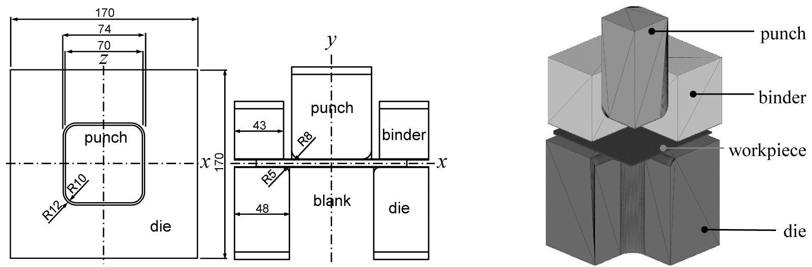
Figure 16.18 Definition of the square-cup deep drawing process
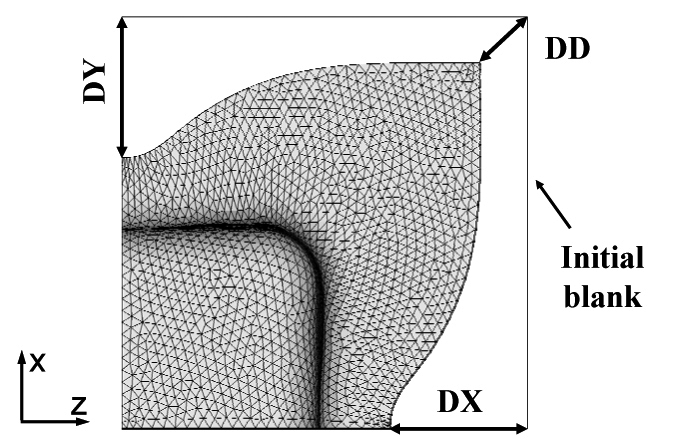
Figure 16.19 Definition of the measured lengths

Figure 16.20 Initial finite element mesh
Figure 16.21 shows the predicted deformation history, and Figure 16.22 shows the predicted final deformed shape and the effective strain. The numerical volume loss that occurred in obtaining these results was 0.256% (single-layer mesh) and 0.483% (two-layer mesh), respectively. These values mean that the numerical uncertainties related to the contact treatment technique and to the penetration of the workpiece into the die and the die into the workpiece were properly controlled (such numerical uncertainty is one of the unfavorable characteristics of volume elements in sheet forming process analysis)...
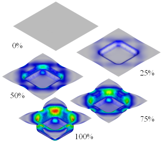
Figure 16.21 Predicted results using the single-layer mesh - deformation history
Figure 10.21 shows the change in the position of the binder, relative to its initial position, as a function of the punch stroke (or as a function of elapsed time). According to this result, the binder moves during forming, and as deep drawing occurs and the workpiece undergoes bending deformation, there is a portion protruding upward from the inside, meaning that the binder load acts mainly on this portion.
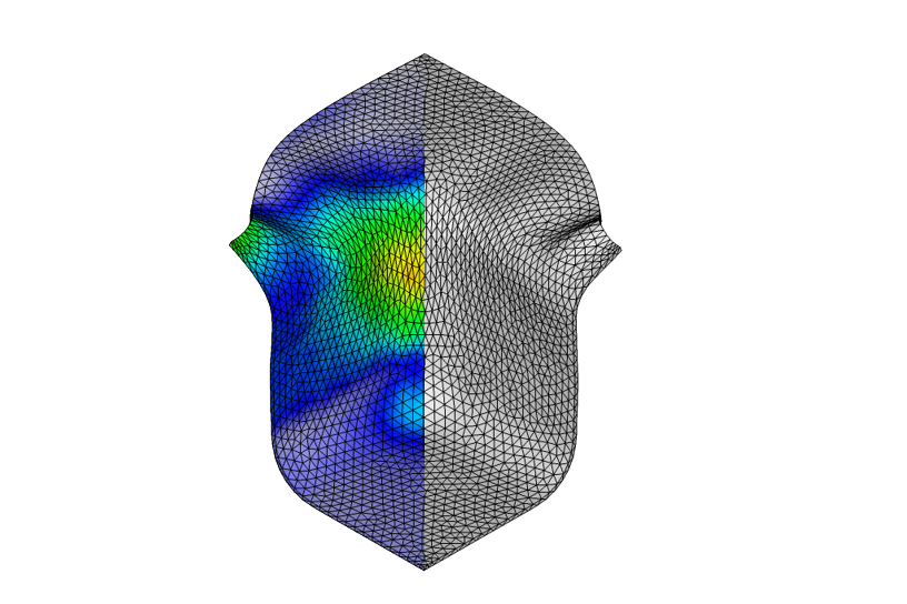
Figure 16.22 Final shape and effective strain distribution
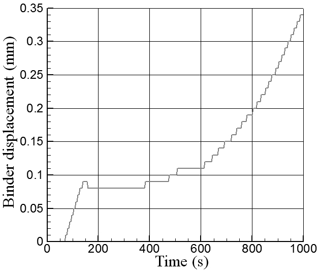
Figure 16.23 Change in binder displacement
Table 16-1 compares the experimental results [16.6] with the predicted results. Broadly similar results were predicted. Even in the rigid-plastic case, engineering meaningful results were obtained despite neglecting the influence of elastic deformation. The elastoplastic analysis results also predicted results close to the experimental values. However, they do not show a large difference from the rigid-plastic analysis results. In this analysis, the anisotropy of the material was not considered. Nevertheless, engineering meaningful results were predicted.
[Table 16-1] Comparison with experimental results and other predicted results [16.7]
| Comparison | DX, DY(mm) | DD(mm) |
|---|---|---|
| Experiment results | 27.95 | 15.36 |
| Tetrahedral-Binder, 1 layer, rigid-plastic | 27.07 | 15.28 |
| Tetrahedral-Binder, 1 layer, elastoplastic | 26.50 | 14.63 |
| Tetrahedral-Binder, 2 layers, elastoplastic | 27.83 | 15.41 |
| Tetrahedral-Binder, 3 layers, elastoplastic | 27.97 | 15.35 |
| Tetrahedral-Binder, 4 layers, elastoplastic | 28.00 | 15.32 |
Figure 16.24 compares the analysis results for DD in Figure 16.19. As can be seen from this figure, when the number of layers is two or more, the results of the elastoplastic volume elements agree better with the experimental values than the results of commercial software using shell elements. When the number of layers increases, the sheet thickness becomes thin so that the aspect ratio of the elements deteriorates, tending to reduce the accuracy of the analysis. Therefore, in the case of this example, considering both analysis accuracy and computation time, a two-layer structure can be judged to be optimal.
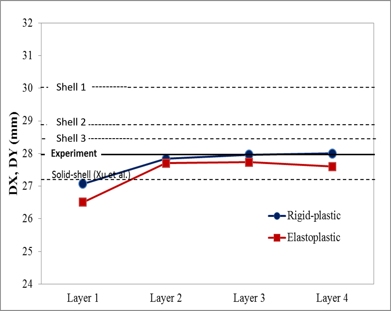
Figure 16.24 Comparison of analysis results and experimental results [16.6, 16.7]
16.5.2.2. Analysis of the Plate Forging Process
Figure 16.25 shows the plate forging process used in this study. This process consists of a punch, a guide, and a blade die below a pad. The pad is supported by a spring. The main process information for the analysis is summarized in Table 16-2. Figure 16.25 shows the initial workpiece shapes of the prediction and the experiment.
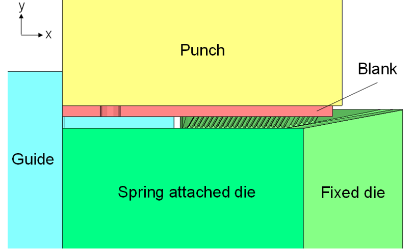
Figure 16.25 Conceptual diagram of the plate forging process
In this analysis, in order to focus on the deformation of the hole, a dense mesh was applied to the rivet hole region with a weighting five times that of the other average mesh. As a result, as shown in Figure 16.26⒜, the mesh can be seen to be densely formed around the hole.
[Table 16-2] Summary of analysis information
| Flow stress of material | $\(\bar{\sigma} = 320 \left( 1 + \frac{\bar{\varepsilon}}{0.00426} \right)^{0.17}\text{ MPa}\)$ |
|---|---|
| Initial material thickness | 3.5mm |
| Friction | Coulomb friction ( $\(\mu = 0.15\)$ ) |
| Spring constant of pad | $\(k = 300.0\text{ N/mm}\)$ |
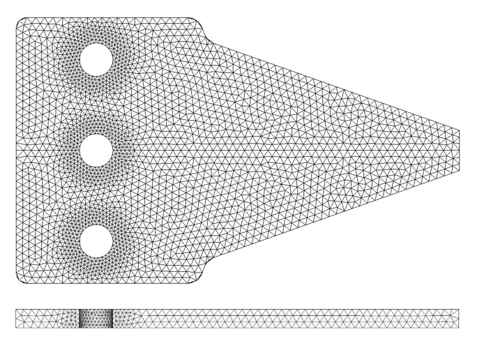
⒜ Initial mesh
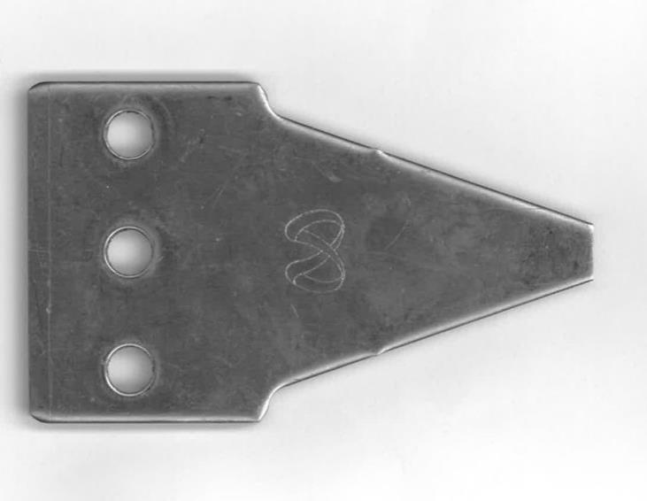
⒝ Initial blank
Figure 16.26 Initial mesh and initial blank
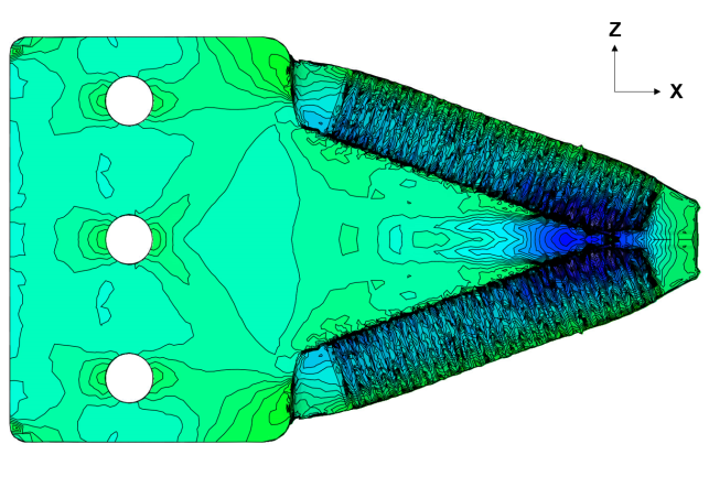
Figure 16.27 shows the strain obtained as an analysis result and the distribution of \(\sigma_{xx}\), which is the direct cause of the deformation of the hole. As shown in the strain distribution of Figure 16.27(a), most of the deformation is concentrated at the blade region. This is one of the general characteristics of plate forging. As shown in Figure 16.27(b), owing to the geometric characteristics of the inclined blade region, the workpiece is pushed toward the guide direction, and a load that resists this is applied to the workpiece. For this reason, compressive deformation occurs in the non-formed region, and this deforms the circular-cross-section hole into an elliptical shape. In particular, it can be confirmed that tensile stress occurs in the \(x\)-direction of the circular-cross-section hole, and compressive stress occurs in the \(z\)-direction.
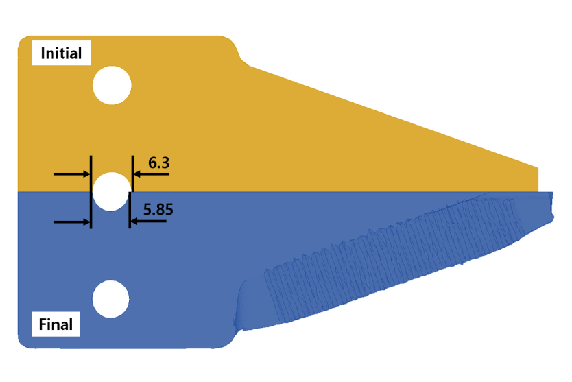
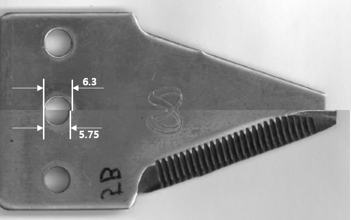
Figure 16.28 compares the analysis results and the experimental results. The experimental value of the dimensional change due to the compressive deformation of the hole region was 5.5 mm, and the predicted value was 4.5 mm. The difference in these results means that the predicted result has engineering significance. It is judged that the difference will be reduced if the anisotropy of the material, the elastic deformation of the die, the rigidity of the side supports, and the like are taken into account.
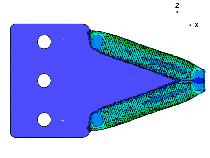
⒜ Effective strain
⒝ Initial blank
Figure 16.27 Main analysis results
⒜ Initial mesh
⒝ Experimental result
Figure 16.28 Deformed shape and hole dimensions
16.5.2.3 Analysis of the Square Deep Drawing Process of Aluminum-Titanium Clad Sheet
The clad sheet forming process analyzed in this section is as shown in Figure 16.29. The clad sheet used is one in which 0.18 mm of titanium is bonded to a 0.4-mm-thick aluminum base material as shown in Figure 16.29. The flow stress of the clad sheet is shown in Figure 16.28. And the Coulomb friction coefficient between the die and the workpiece was assumed to be 0.12.
Using symmetry, 1/2 of the entire analysis domain was considered as the analysis target; the total number of layers was set to six, and the base material was divided into three layers as shown in Figure 16.31. The total number of elements is 150000. The blank holding force is 25 kN, and this was handled by the load-application die technique [16.8]. The speed dependence of the material was neglected, and as a result, the descending speed of the punch was assumed to be 1 mm/s.
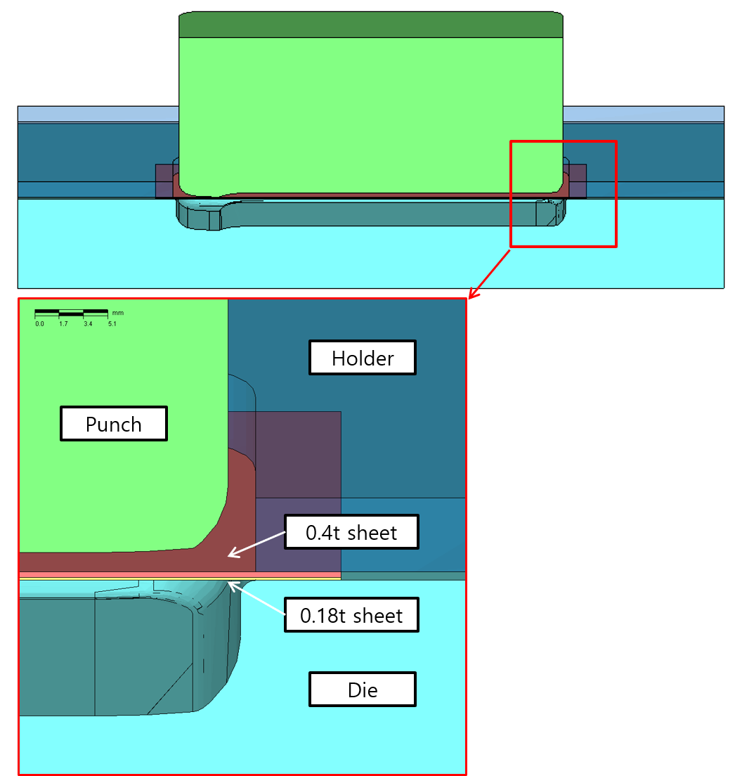
Figure 16.29 Clad sheet forming process diagram
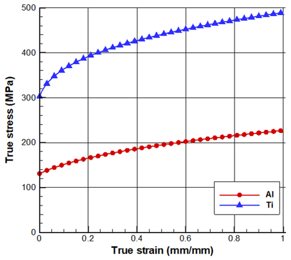
Figure 16.30 Flow stress
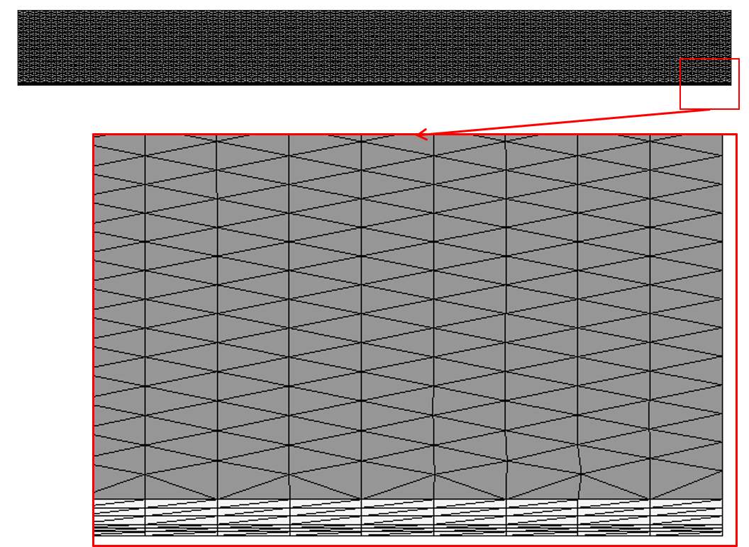
Figure 16.31 Initial mesh
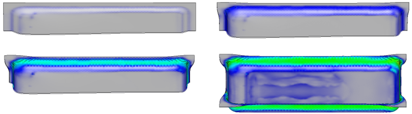
Figure 16.32 Deformation history
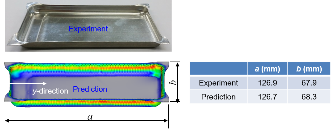
Figure 16.33 Comparison of experimental results and analysis results
16.5.2.4 Analysis of the Oil Pan Forming Process
As shown in the conceptual diagram of the oil pan forming process in Figure 16.34, the components that make up the process are the material, the punch, the lower die, the blank holder, and the like. Analyses using volume elements (tetrahedral element (AFDEX 3D) and hexahedral element [16.9]) and plate elements were performed. Considering symmetry, 1/2 of the entire domain was considered as the analysis domain.
The material is A5754 sheet, and the blank holder force is 20 tons. A hybrid friction law was used as the friction law, and the Coulomb friction coefficient was assumed to be 0.125 and the friction constant 0.375. The speed dependence of the material at room temperature was neglected.
Figure 16.35 shows the deformation history and the strain distribution obtained by the tetrahedral element and the elastoplastic finite element method. Figure 16.36 shows the thickness distribution, and comparing Figures 16.34 and 16.35⒞, it can be seen that the minimum-thickness point and the maximum-effective-strain point are different. At the maximum-strain point, the thickness was found to have increased due to compressive deformation.
As shown in Figure 16.36, the two results using volume elements are almost identical from the standpoint of minimum thickness. The thickness difference is 0.005 mm. On the other hand, the difference between the plate element result and the volume element result reaches about 0.05 mm. However, overall, the two results are similar. In Figures 16.36⒜ and ⒝, the plate element and the hexahedral element represent the thickness distribution with the same color scheme, whereas the tetrahedral element in Figure 16.36⒞ uses a different color scheme. For this reason they appear different, but the actual numerical comparison results are very similar.
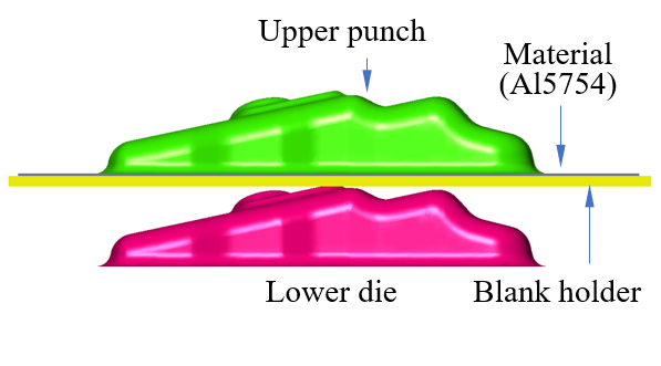
Figure 16.34 Conceptual diagram of the oil pan forming process
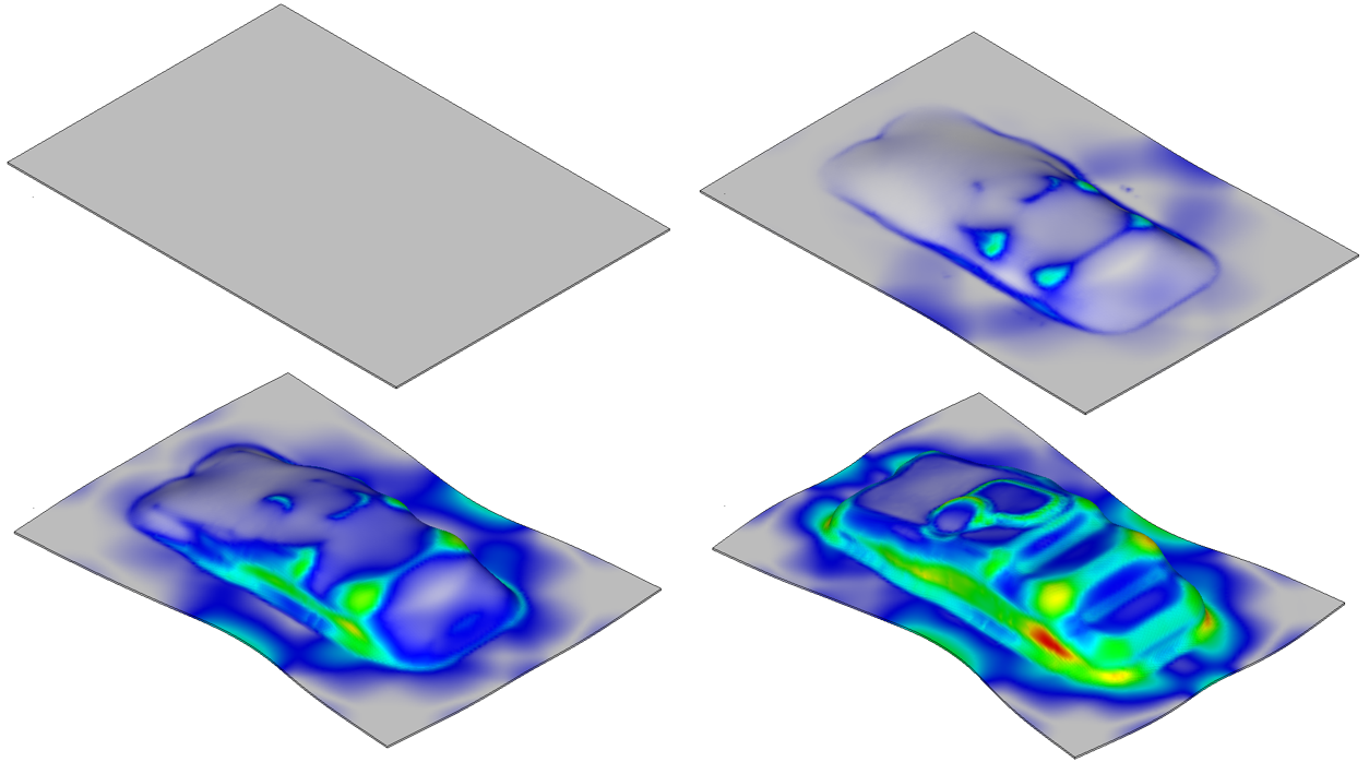
Figure 16.35 Analysis results using the tetrahedral element (strain)
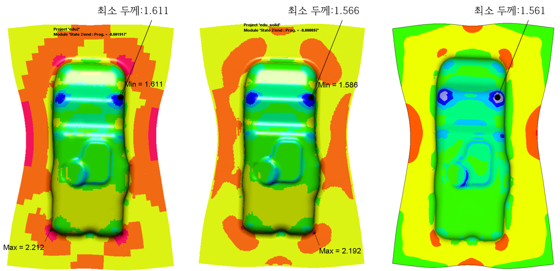
Figure 16.36 Comparison of analysis results using volume elements and plate elements
16.6 Forming Limit Diagram
16.6.1 Definition of the Forming Limit Diagram
The forming limit diagram (FLD) is an indicator for evaluating the formability of a workpiece, and it is used in the sheet metal forming field as a guideline for evaluating formability and as a diagnostic criterion for forming failure. It represents the deformation region allowed for the sheet, taking the local necking during sheet metal forming as the useful limit strain, with the major strain on the vertical axis and the minor strain on the horizontal axis.
As shown in Figure 16.37, when a circle of diameter \(d_0\) engraved on the sheet surface before forming is deformed into an ellipse with a major-axis length of \(d_1\) and a minor-axis length of \(d_2\) due to deformation, the major strain \(\varepsilon_1\) and the minor strain \(\varepsilon_2\) of the sheet are defined by the following equations.

Figure 16.37 Definition of major strain and minor strain
The major strain and minor strain can have various combinations depending on the deformation state. Figure 16.38 shows the signs of the major strain and minor strain for each deformation state.
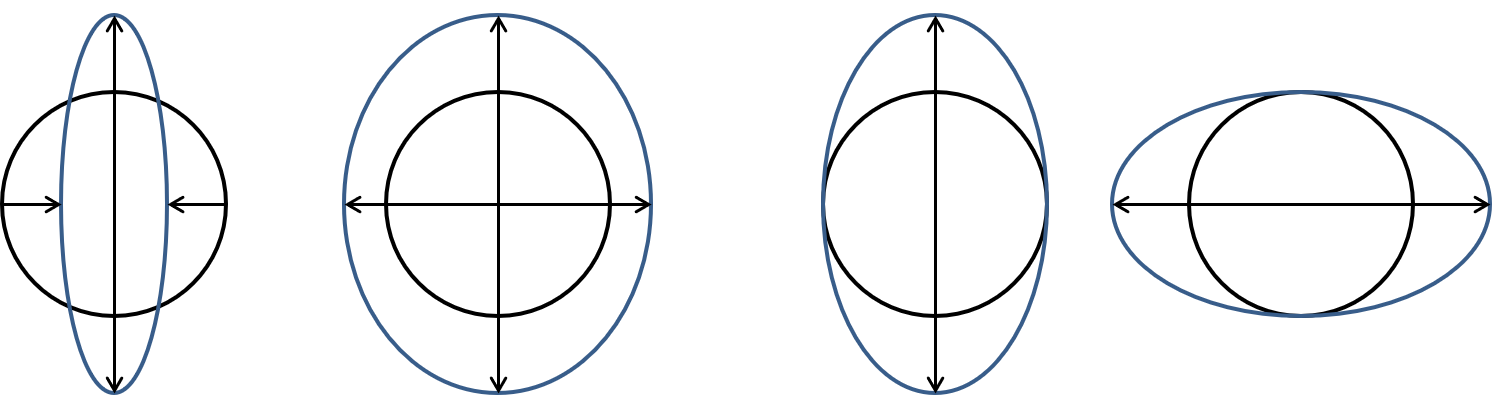
Figure 16.38 Signs of major strain and minor strain by deformation state
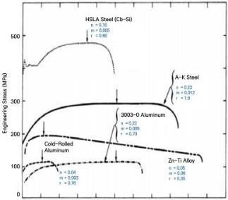
Figure 16.39 shows the forming limits on the uniaxial tension curves of various metallic materials. As shown in this figure, metals exhibit various forming limits, and in general, materials with high strength tend to have low elongation. However, there are cases, such as the A-K alloy, that have both high strength and high elongation. In general, when the maximum load is reached in a tensile test and necking begins, local deformation proceeds and rapidly leads to fracture. However, in the cases of A-K, Zn-Ti, and Al3003, cases are observed in which elongation proceeds gradually from the maximum load until fracture.
Engineering strain
Figure 16.39 Uniaxial tensile test curves and forming limits
16.6.3 Major Forming Limits in Sheet Metal Forming
16.6.3.1 General Sheet Metal Forming Modes
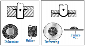
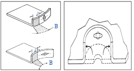
Figure 16.40 shows the general plastic forming modes of metal sheets. For example, Figure 16.40⒜ shows the drawing mode. In the drawing mode, the flange region, wall region, and bottom region undergo different deformations. Figures 16.40⒜, ⒝, ⒞, and ⒟ are different plastic forming modes and undergo different deformation histories. Therefore, the fracture strain differs for each region of a plastic forming mode, and it is not easy to predict this in the field. Accordingly, fracture is predicted using empirical knowledge based on many experiments, or fracture is predicted using the finite element method. In the finite element analysis of a sheet metal forming process, if the coordinates of the calculated strains, that is, the major strain and minor strain, lie above the fracture curve on a forming limit diagram prepared in advance through experiments, it means that the material fractures.
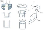
Figure 16.41 conceptually shows a case in which forming is limited by fracture that occurs in the tensile deformation mode during the deep drawing process and by wrinkling and thickness reduction that occur under the compressive deformation mode. Therefore, the key in the design of a drawing process is to prevent wrinkling in the flange region and to prevent fracture due to excessive thickness reduction in the wall region. The example on the left of Figure 16.42 shows wrinkling occurring during forming, with a region where the combination of strains falls in the upper part of the forming limit diagram. The figure on the right shows the strain distribution obtained through optimal process design. As shown in the figure, through optimal process design it is possible to improve wrinkling while having all regions of interest located in the lower part of the forming limit diagram.
⒜ Drawing mode ⒝ Stretching mode
⒞ Flanging mode (d) Burring mode
Figure 16.40 Fracture by plastic forming mode
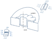
⒜ Deep drawing process ⒝ Wrinkling and fracture
Figure 16.41 Occurrence of wrinkling during drawing and fracture due to thickness reduction in the wall region
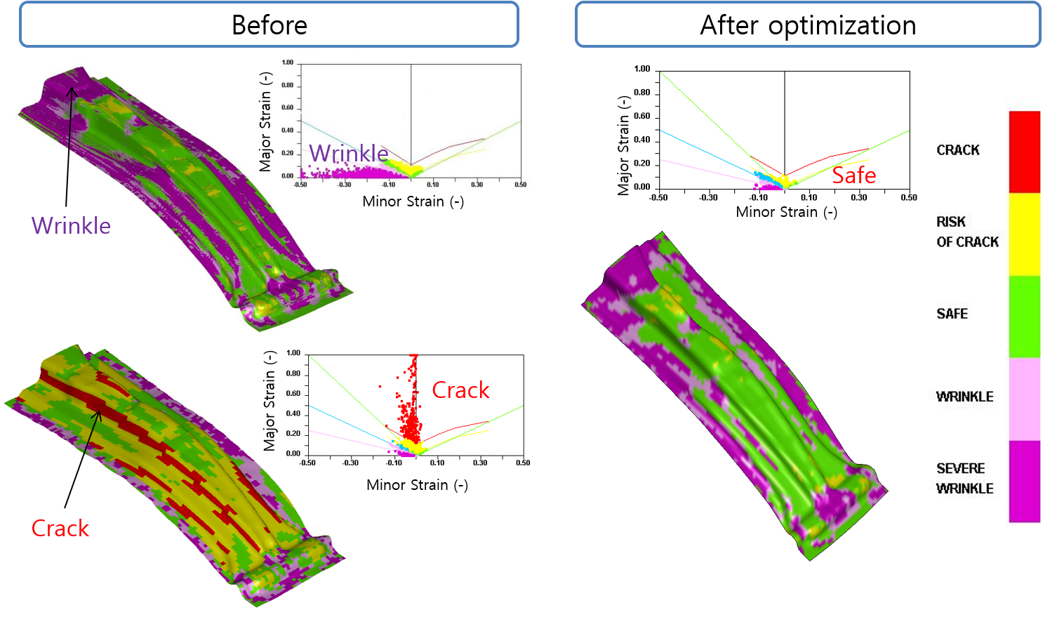
Figure 16.42 Prevention of wrinkling and tearing through optimal die design
16.6.3.2 Evaluation of Deep Drawability
The LDR (Limit Drawing Ratio) is defined in the deep drawing mode as the ratio of the blank diameter \(D_b\), which can be drawn to the maximum without tensile fracture of the material, to the punch diameter \(D_p\). That is,
This value is used to determine the number of drawing operations. The LDR is determined at the limiting condition of no tearing by performing a deep drawing test while keeping the BHF (blank holder force) constant, as shown in Figure 16.41(a).
Meanwhile, the deep drawability can also be predicted by a theoretical method. The assumptions for developing the theory are summarized as follows. (1) The cup drawing process is assumed to be an axisymmetric problem. (2) It is assumed that a plane strain state of \(d\varepsilon_3 = 0\) is maintained at the flange region, and a plane strain state of \(\sigma_3 = 0\), \(d\varepsilon_2 = 0\) is maintained at the cup wall. (3) The material is regarded as normally anisotropic, and strain hardening is neglected. (4) Hill's quadratic anisotropic yield theory is followed.
The axial stress \(\sigma_1\) that must be supported at the cup wall is
Here, \(\sigma_1\) is the axial stress, and \(\sigma_f\) is the yield stress of the flange region where \(d\varepsilon_3 = 0\).
Since strain hardening can be neglected, once yielding occurs at the cup wall, the cup immediately fractures by necking. If the yield stress at the cup wall, where \(\sigma_3 = 0\), \(d\varepsilon_2 = 0\), is denoted by \(\sigma_w\), the drawing limit is determined when \(\sigma_1\) becomes equal to \(\sigma_w\). That is,
From Hill's quadratic anisotropic yield condition, \(\sigma_f (d\varepsilon_3 = 0)\) and \(\sigma_w (d\varepsilon_2 = 0, \, \sigma_3 = 0)\) are, respectively,
Here, \(R\) is the anisotropy coefficient.
Therefore, the \(\text{LDR}\) is obtained by the following equation.
If Hosford's anisotropic yield condition is followed, the LDR is summarized by the following equation.
Here, \(\eta\) is the deformation efficiency considering bending deformation and frictional work, usually having a value between 0.74 and 0.79.
16.6.4 Construction and Evaluation of the Forming Limit Diagram
16.6.4.1 Forming Limit Curve
The FLD is a chart that represents the strain state at various points of the blank on the major strain axis and the minor strain axis, and it is called the forming limit diagram. It is a plot obtained by measuring all the various strain states of various specimens. The blanks obtained in the experiment are examined and classified into those in which fracture occurred, those in which necking occurred, and those that are safe, and are marked on the FLD. For various specimens, the line drawn by finding the boundary that distinguishes fracture from necking at these marked measurement points is called the forming limit curve, or FLC (Forming Limit Curve). Figure 16.43 shows an example of a typical FLC. That is, with this line as the boundary, if the strain state is located above it, it is exposed to fracture, and if it is located below it, it is judged to be safe.
Meanwhile, several factors influence the construction of the FLC. Friction has a great influence on the magnitude and location of the strain at the point where fracture occurs. There is also an error associated with measuring a curved-surface region to evaluate strain. There are also several types of formability evaluation test methods, and differences arising from these also exist. Therefore, the marginal curve is one in which a safe region is set considering these error factors. As shown in Figure 16.43, it is common to set this marginal curve 10% below the FLC.
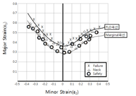
Figure 16.43 Forming limit curve and marginal curve
The FLC represents the fracture limit strain of a sheet material under various deformation modes (biaxial tension, uniaxial tension, plane strain, compressive deformation, etc.). The FLC is also greatly affected by the material thickness. Looking at the FLC of the sheet in Figure 16.44, it can be confirmed that the formability differs according to various deformation modes. If the FLC of a material is determined in an experiment that varies the strain linearly, formability can be judged from the FLD. However, in a sheet metal forming process, the change path of the strain in all regions is nonlinear. When setting the safe region, taking this into account, the marginal curve is sometimes set 5 to 20% below the FLC. Figure 16.44 shows the correlation between the deformation mode and the forming limit curve.

Figure 16.44 Deformation modes of the sheet and the forming limit curve in the FLD
16.6.4.2 Measurement of Sheet Deformation
In the case of a sheet, the stress in the thickness direction is negligible. That is, by assuming \(\sigma_3 = 0\) and \(\tau_{13} = \tau_{23} = 0\), it can be treated as a plane stress problem. Therefore, only the two principal strains (\(\varepsilon_1\), \(\varepsilon_2\)) acting on the plane of the sheet are measured, and the strain in the thickness direction (\(\varepsilon_3\)) is calculated using the law of volume constancy of plastic deformation.
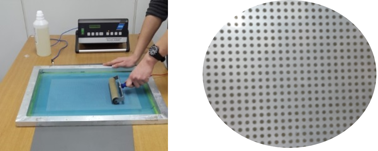
⒜ Etching of the circular grid on the sheet ⒝ Circular-grid sheet
Figure 16.45 Circular-grid sheet for FLD measurement
The circular grid method of Figure 16.45 is used as the method of measuring the principal strains. In the circular grid method, after marking a circular grid on one side (the product outer surface) of the sheet, a dome stretching test or a press forming (sheet deformation) test is performed. The marked circle is deformed into an elliptical shape by the test. This shape change is quantified by measuring the lengths and directions of the major and minor axes of the ellipse using a measuring instrument or optical measurement equipment, as shown in Figure 16.46. That is, the major strain and minor strain can be obtained from Equations (16.1) and (16.2).

Figure 16.46 Deformation of the grid and determination of the major and minor strains
16.6.4.3 Example of Forming Limit Diagram Construction
Figure 16.47 shows the shapes of machined specimens with different widths. The prepared specimens are used to determine the FLD curve by measuring the major strain and minor strain at fracture for each specimen through the FLD test equipment of Figure 16.48. The test equipment consists of an FLD specimen, a punch, and a holder, and by measuring images from the top through two CCD cameras while deformation proceeds, the major strain and minor strain of each part are calculated from the start of deformation through necking to fracture and plotted on the plane of the major strain axis and minor strain axis. Figure 16.49⒜ shows the shape of the initial specimen and the shape of the specimen after deformation, and the strain distribution of the material deformed by the dome-shaped punch is shown in Figure 16.49⒝.
From the plot of major strain and minor strain constructed from the experiment, the FLC can be determined, as shown, for example, in Figure 16.50. Therefore, for a combination of strains occurring in an actual forming process, if the finite element analysis result also lies in the upper part of the forming limit curve, it is judged that fracture occurs, and if it lies in the lower part, it is judged to be safe.
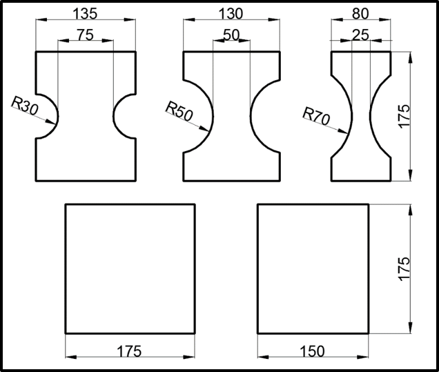
Figure 16.47 Fabrication of specimen shapes with various widths for forming limit diagram testing
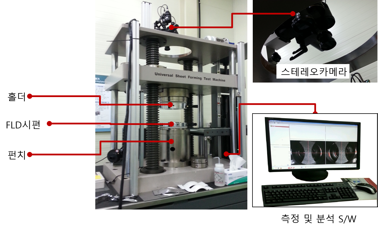
Figure 16.48 Forming limit diagram test equipment and optical measurement equipment for strain measurement
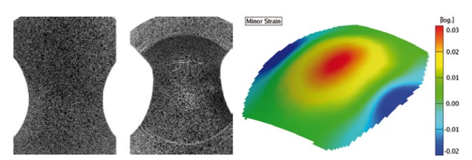
Figure 16.49 Strain calculation using optical measurement S/W after FLD measurement
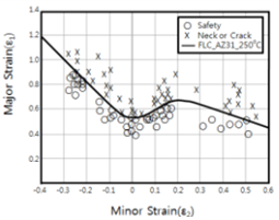
Figure 16.50 Fracture of the sheet according to the strain on the forming limit diagram
16.6.5 Theoretical Approach to the FLD
Since it is practically difficult to derive the FLD experimentally for all steel sheets, a method using a representative FLD has been proposed. In this method, using the limit plane strain FLC0 (plane strain intercept), which is the lowest point on the FLC obtained from experiment or a theoretical equation, the FLC of the steel sheet is obtained by shifting the representative FLC in the major strain axis direction to the FLC0 point. As the representative FLC, the Keeler-Goodwin curve [16.10, 16.11] or the FLC for AK cold-rolled steel sheet presented by Hecker [16.12] is used. The magnitude of FLC0 depends on the material thickness, the work-hardening exponent, the elongation, the yield stress, and the like, and NADDRG recommends the following empirical equation for the case of \(n < 0.21\).
Here, \(n\) is the work-hardening exponent and \(t\) is the thickness of the sheet.
The FLC curves in the first and second quadrants of the FLD are approximated by the following equations, respectively.
Here, \(e_1\) and \(e_2\) are the major strain and minor strain expressed as percentages, respectively. In actual situations, since the difference between the true strain and the nominal strain is not large, they are sometimes not distinguished. However, since these approximate equations are based on experiments and used nominal stress, the relationships between \(e_1\) and \(e_2\) and the major strain and minor strain are as follows.
16.7 Cause of Fracture Occurring During the Thick-Plate Forging Process of Clad Material
Figure 16.51 shows the experimental result of thick-plate forming of a clad material in which 0.6 mm of titanium is bonded to a 3.4-mm-thick aluminum base material [16.13]. The flow stresses of the base material and the composite are shown in Figure 16.30. The Coulomb friction coefficient between the die and the workpiece was assumed to be 0.06.
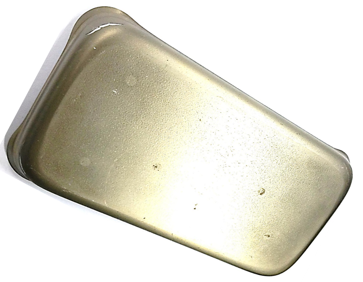
⒜ Overall shape
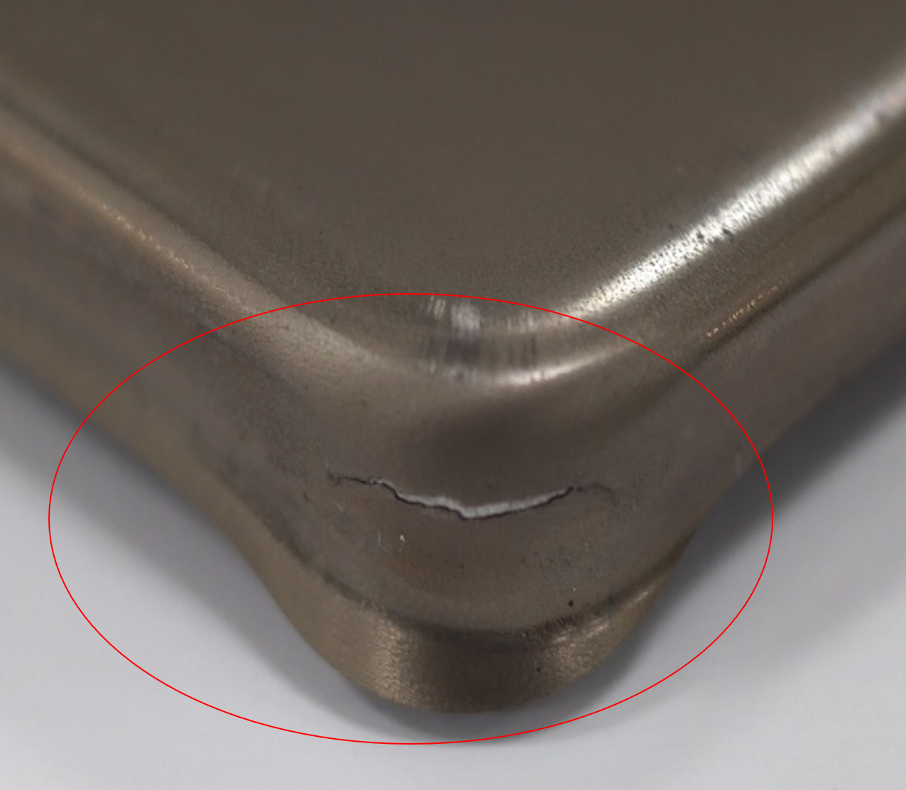
⒝ Enlarged fracture region
Figure 16.51 Experimental result
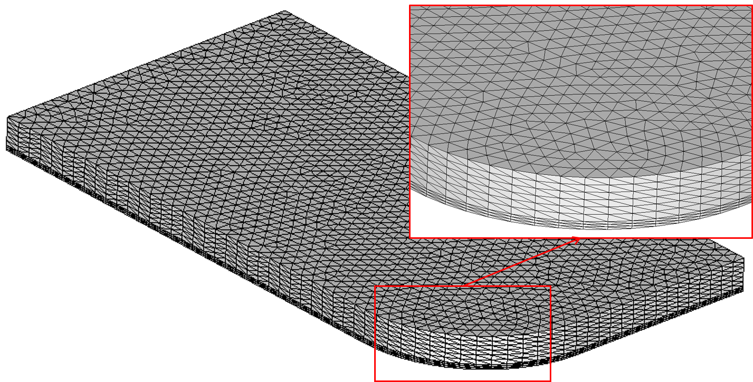
⒜ Finite element mesh of the initial workpiece
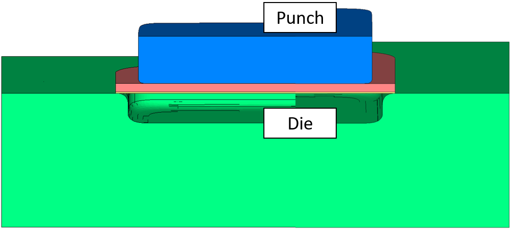
⒝ Conceptual diagram of the process
Figure 16.52 Finite element analysis model
To reflect the influence of the thickness direction, the finite element model used a layered-element technique suitable for the forming analysis of clad materials, as shown in Figure 16.52. Considering the negative influence of remeshing that occurs during the analysis, that is, numerical smoothing and intractability, the quality of the initial mesh was improved, and elements causing various numerical errors were removed.
The FLD curve used for fracture evaluation is as shown in Figure 16.53 [16.14]. Taking the limit major strain with respect to the minor strain as the reference, the percentage of the major strain was defined as the FLD index.
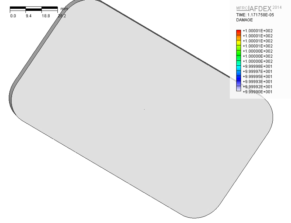
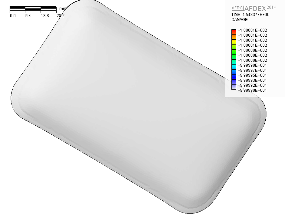
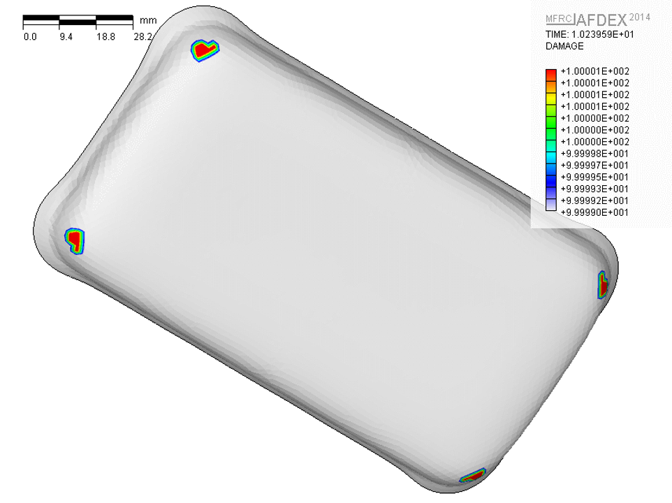
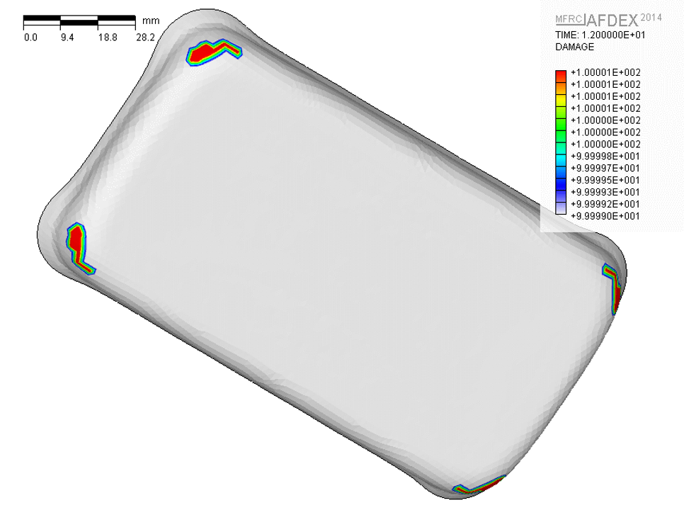
Figure 16.54 shows the deformation history together with the process of change of the FLD index exceeding 100. The overall appearance of the predicted result agrees well with the experimental result of Figure 16.51. The FLD index for a given major strain and minor strain was defined as the percentage of the major strain with respect to the limit value of the major strain obtained at the minor strain from the forming limit curve. Therefore, when the FLD index reaches 100.0, it means that fracture occurs. In the case of this process, as shown in Figure 16.54, fracture occurs upon reaching 1.0 second, and thereafter the fracture grows as shown in Figure 16.51. This can be seen from the analysis result of the forming limit diagram of Figure 16.55. Around a minor strain of 15%, the major strain of many elements already lies in the upper part of the forming limit curve. That is, fracture occurred before the end of forming.
Therefore, the slight difference between the maximum value of the FLD index in Figure 16.54 and the fracture location in Figure 16.51 is due to the aforementioned reason. Considering this point, in Figure 16.54, the upper boundary at which an FLC index exceeding 100.0 first appears at the end of forming should be regarded as the actual fracture point. This agrees with the fracture point confirmed in the experiment.
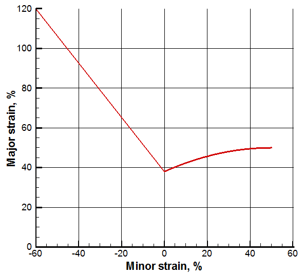
Figure 16.53 Applied forming limit diagram [16.14]
(a) t = 0.0s
(b) t = 0.45s
(c) t = 1.0s
(d) t = 1.2s
Figure 16.54 Change of the FLD index according to stroke
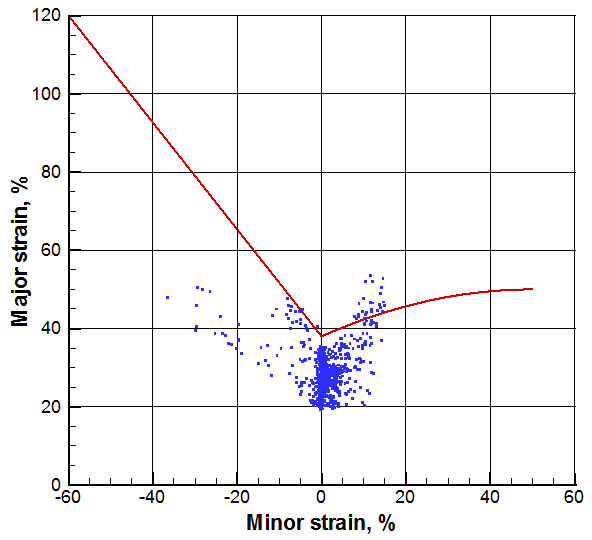
Figure 16.55 FLD analysis result