15 Optimal Design of Metal Forming Processes and Variables
15.1 Forming Load Optimization
15.1.1 Hot Forging Process
One of the elements emphasized in the design of metal forming processes is the forming load. This is because the forming load is directly connected to cost. In general, a process design that minimizes the forming load is highly likely to be advantageous in terms of quality as well. This is because the forming load and the forming energy are in a functional relationship. In manufacturing a certain metal-formed product, if much energy is consumed despite the same working conditions, the difference in energy can cause excessive deformation of the material.
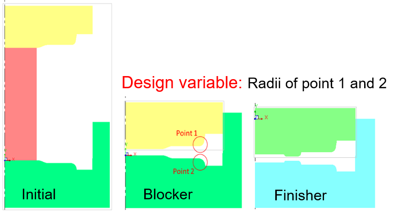
Figure 15.2 Change of the forming load of the piercing process according to the improvement of the design
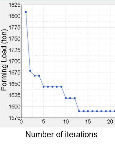
Figure 15.3 Change of the effective strain and forming load of the optimal design
15.1.2 Maximization of the Holding Load of the Clinching Process
Figure 15.4 shows the clinching process and the separation process. Because this process aims to join two sheets, strength at the time of separation is required. This strength depends on the neck thickness and the undercut defined in Figure 15.4(a). Since these two elements depend on the deformation characteristics of the material, optimal design based on prediction technology is important.
Figure 15.5(a) defines the design variables. There are a total of 5 design variables. Figure 15.5(b) shows the optimal design process of the strength. Figure 15.4 shows the process of change of the effective strain when the optimal conditions are used.
In the initial design the maximum holding load was about 3500 N, but the maximum holding load of the optimal design reached 4970 N, and until this result was obtained, a total of 15 iterations of design and analysis were carried out.

Figure 15.4 Clinching process and separation process
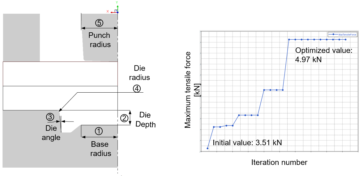
Figure 15.5 Design variables and convergence characteristics
15.2 Quantification of Grain Flow Lines
Ito et al. [15.1] studied the life of tapers for tapered roller bearings. According to their research results, summarized in Figure 15.6, it can be seen that the direction of the grain flow lines of the taper has a critical influence on the life. Depending on the direction of grain flow line formation, the life differs by up to more than 6 times.
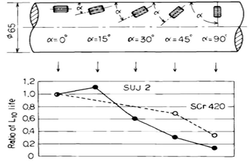
Figure 15.6 Importance of grain flow lines
15.7 is a failure case of a first-generation hub bearing outer race produced by hot forging [11.7]. The external appearance of this forged product has no problem, but it is a case that failed due to a grain flow line defect. In this figure the left side shows the experiment and the right side shows the predicted result. This case is an example sufficient to emphasize the importance of grain flow lines (grain flow, metal flow lines) in forged products.
Figure 15.7 First-generation bearing outer ring
Figure 15.8 is a figure concerning the forging of a flanged outer ring. Figure 15.8(a) shows the grain flow lines of the product before Figure 15.8(b) was developed and the predicted result for it. It can be seen that the grain flow lines of the improved product are surface-friendly in the region where the steel ball contacts. This example, together with the importance of grain flow lines, tells of the difficulty of designing a forging process that considers grain flow lines.
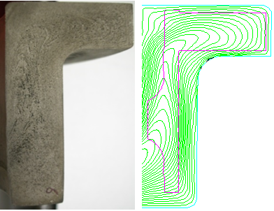
(a) Conventional process
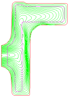
(b) Optimized process
Figure 15.8 Flanged bearing outer ring
These grain flow lines are predicted by two methods. The first is a method in which a point cloud and a set of line segments connecting these points are input initially and those points are tracked. The second is a method in which the initial positions of the finite element nodes are calculated as a kind of nodal value, and the points whose initial nodal coordinates are identical are connected. The former has nothing but geometrical information. It merely tracks and displays a kind of grid input upon request. The latter is expressed mathematically, and useful information can be obtained through post-processing. The grain flow lines of Figures 15.7 and 15.8 are examples of the former, and Figure 15.9 is an example of the latter.
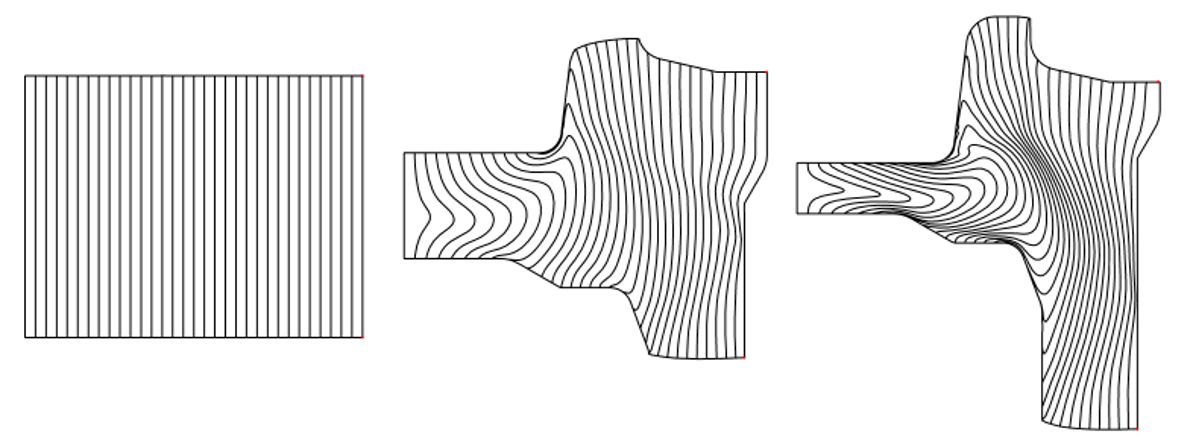
Figure 15.9 Visualization of grain flow lines by the mathematical approach
It is worth noting that the grain flow lines of Figure 15.9 have the same \(x\) coordinate. Therefore, the grain flow line is expressed as a function of the initial coordinates. This function is a vector function. That is, at one point the function has two or more values (two in two dimensions, three in three dimensions). Let this function be
and it is called the grain flow line function.
As seen in Figure 15.10, the curves or surfaces on which each component of this vector function has a constant value are directly or indirectly connected to the grain flow lines, and the direction of their gradient is perpendicular to the grain flow lines and the magnitude means the density of the grain flow lines. Therefore, the gradient of the grain flow line function is defined as the grain flow line density. And the gradient of the grain flow line density is a second-order tensor, that is, an overlap index can be defined from the grain flow line tensor.
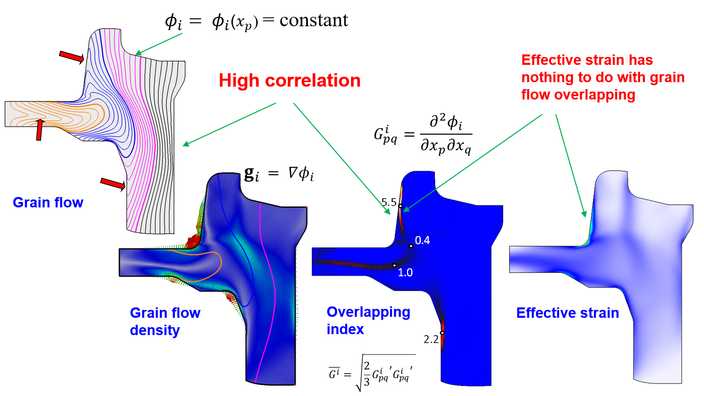
Figure 15.10 Quantification of grain flow lines
The grain flow line density (Equation 15.2), the grain flow line tensor (Equation 15.3), and the overlap index (Equation 15.4) are mathematically defined as follows.
As seen in Figure 15.10, it can be confirmed that the grain flow line density function \(g_i = \nabla \phi_i\) quantitatively expresses well the actual density of the grain flow lines. And the distribution of the grain flow line overlap index \(\bar{G}^i\) well represents the degree of overlap of the grain flow lines. However, it can be seen that the effective strain distribution is unrelated to the degree of overlap of the grain flow lines. Figures 15.11 and 15.12 show the quantified values of the grain flow lines calculated during the hot forging process analysis of a crankshaft and a connecting rod.
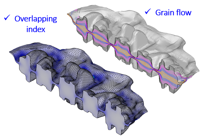
Figure 15.11 Quantification of grain flow lines of the crankshaft hot forging process
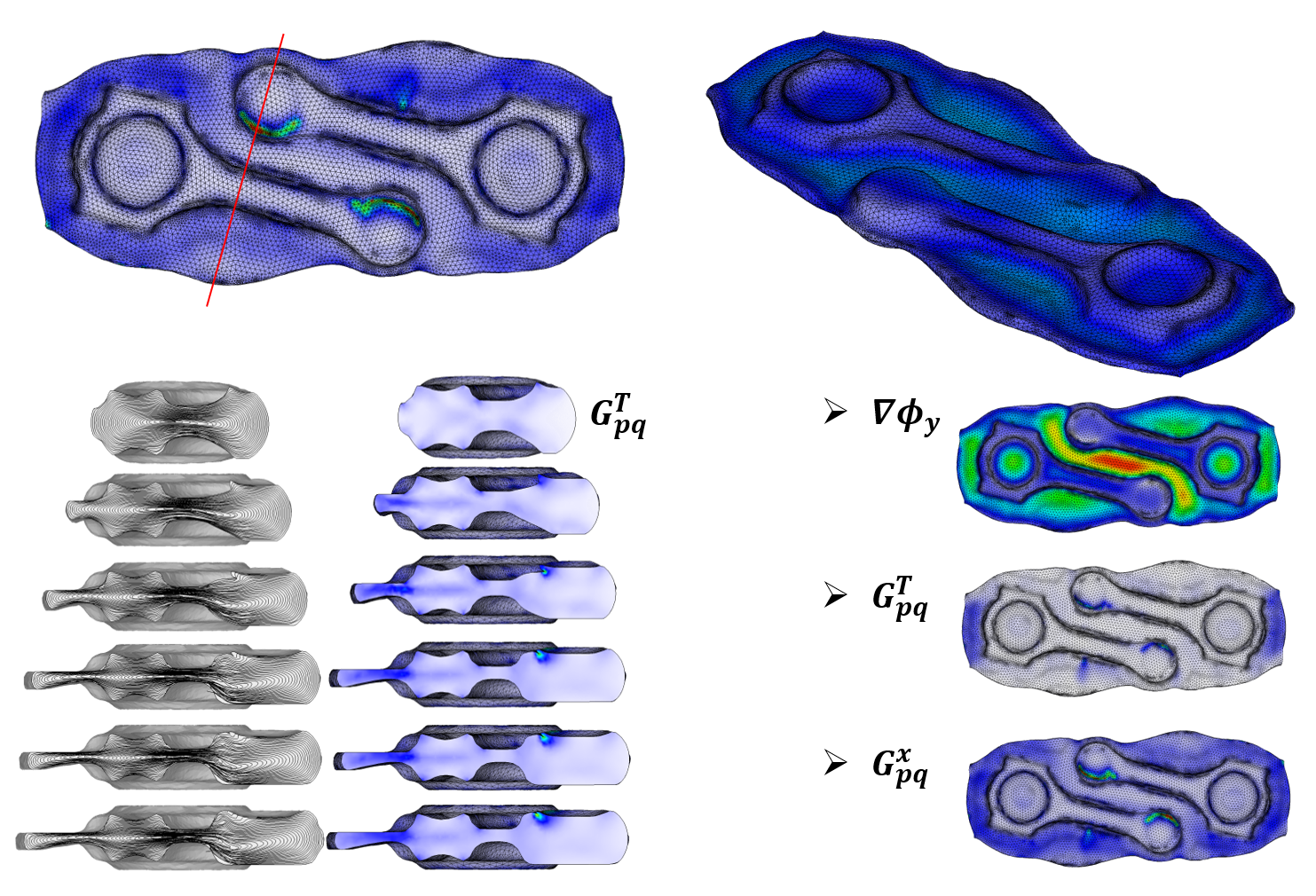
Figure 15.12 Quantification of grain flow lines of the crankshaft hot forging process
15.3 Optimal Design Considering Grain Flow Lines
Over the past 30 years the analysis technology of metal forming processes has developed rapidly, and the use of related software has become essential. A characteristic of metal forming processes is that they apply plastic deformation to a solid to make it into a desired product, and there is an aspect in which the creative elements of the engineer determine the success or failure of the process. Simulation technology for metal forming processes has made numerous contributions to solving such characteristic problems.
Metal forming optimization technology has also been studied for a long time, but there have been clear limits to its application due to various factors. One of the causes is that there are limits to considering the grain flow lines emphasized in the industrial field. Most existing research has only minimized the load or considered strain and its derived state variables. As explained in Section 15.2, a technique for quantifying grain flow lines was recently developed. By using this technology, since the quality of the grain flow lines can be expressed numerically, the way to optimal design considering grain flow lines has been opened.
This section introduces three cases of optimal design.
15.3.1 Optimal Process Design Using the Grain Flow Line Function
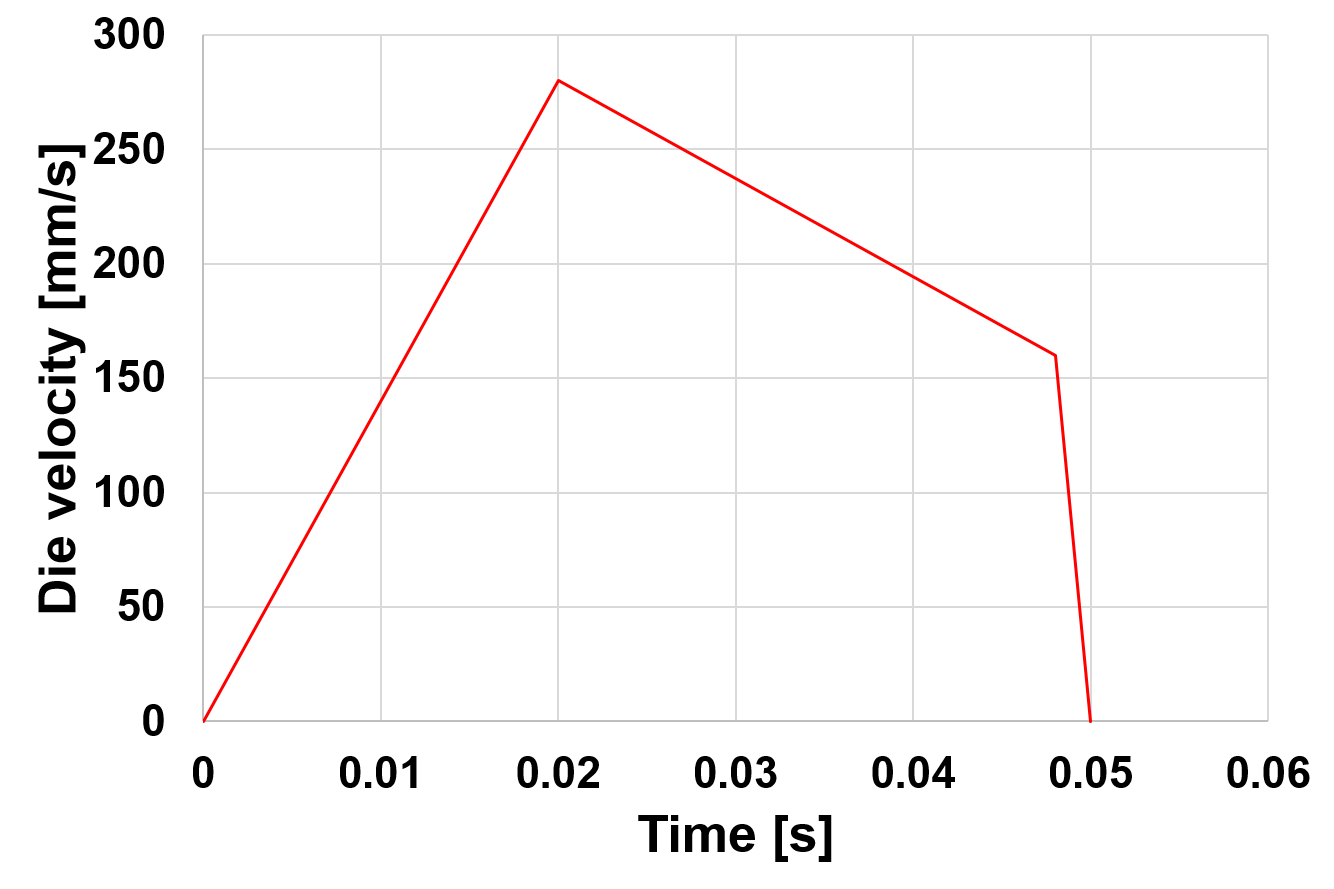
Figure 15.13 shows the 3-stage first-generation hub bearing forging process under study and the design variables. The stroke distance (s) of the blocker process is defined as the design variable. The material is STB2 [12.2]. The die velocity is 200 mm/s, and the friction coefficient between the die and the workpiece was assumed to be 0.2.
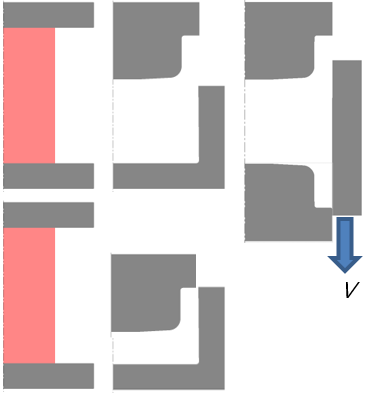
Figure 15.13 Forging process and design variables
To satisfy the up-down symmetry of the grain flow lines of the bearing outer ring, minimization was performed with the difference between point P1 and point P2 defined as the objective function, as seen in Figure 15.14. That is, the objective function is as follows
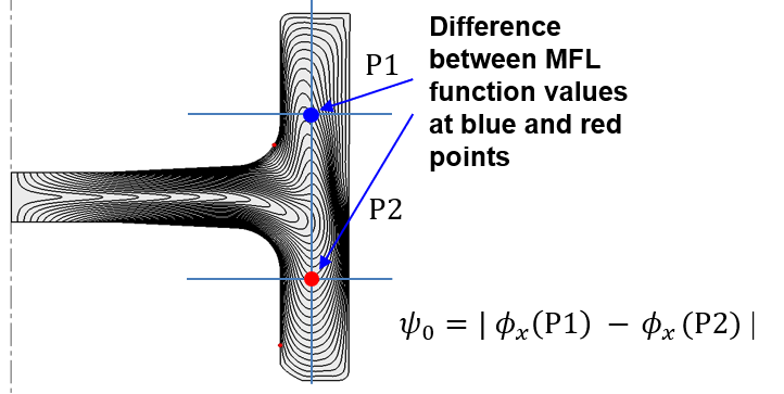
Figure 15.14 Occurrence of asymmetric grain flow lines and definition of the objective function
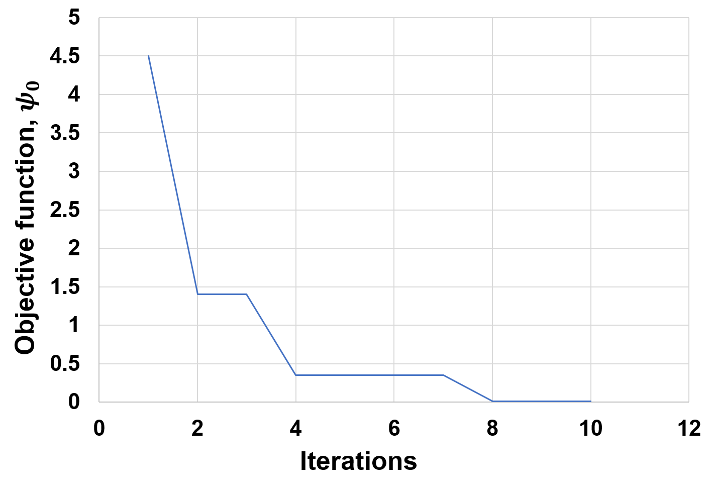
Figure 15.15(a) shows the optimal velocity profile, and Figure 15.15(b) shows the process of optimization, that is, the convergence characteristics of the solution. Figure 15.16(a) is the analysis result before the process optimization design, and Figure 15.16(b) shows the optimized process analysis result. As can be seen from the optimal design results, it is judged that grain flow line optimization technology can be applied quite usefully.
(a) Optimal velocity profile
(b) Convergence characteristics
Figure 15.15 Optimal design and convergence characteristics
15.3.2 Optimal Process Design Using the Grain Flow Line Density
Using the surface normal direction of the product and the grain flow line density vector in Figure 15.17, the grain flow line discontinuity index (surface affinity index) was defined as follows. That is, it means that the more the direction of the grain flow line density vector coincides with the direction of the outward normal vector at the product surface, the more desirable it is. Therefore, the following equation was used as the objective function.
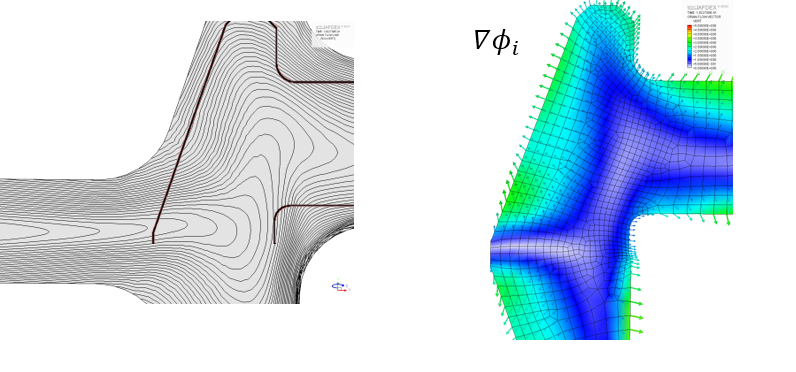
Figure 15.17 Definition of the objective function
Figure 15.18 shows the grain flow lines of the 3-stage hot forging process of the outer ring of a flanged tapered roller bearing, that is, the hot forging process of the upsetting, blocker, and finisher processes of the initial design. As seen in Figure 15.18(b), it can be seen that the grain flow lines are poor in the region where the tapered roller contacts. That is, the grain flow lines undergo severe discontinuity in the region where the tapered roller contacts. Therefore, quality-considering optimization was performed with Equation (15.6) as the objective function
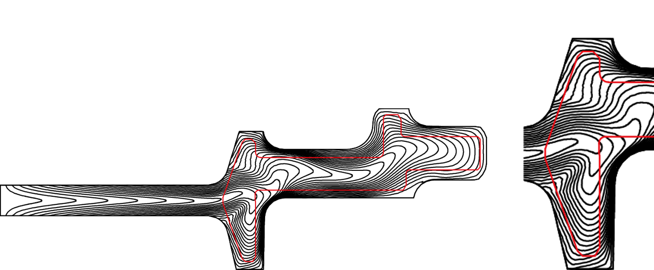
Figure 15.18 Initial design of the forging process of the flanged tapered roller outer ring

Figure 15.19 Definition of design variables
Figure 15.19 defines the design variables of the blocker process. Among the upper and lower die shapes, \(b_1\), \(b_2\), \(b_3\) were selected as design variables, and optimization was performed using the objective function of Equation (15.6). Figure 15.20 shows the change of the blocker die shape through optimization compared with the initial design and the degree of improvement of the grain flow line discontinuity phenomenon, and it can be confirmed that the grain flow line discontinuity phenomenon is improved in the region of interest, that is, the inclined region where the tapered roller contacts.
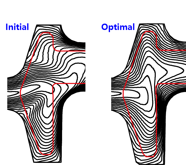
Figure 15.20 Comparison of the initial design and the optimal design
15.3.3 Optimal Process Design Using the Overlap Index
Figure 15.21 shows a pulley-type axial hot forging process. Such a pulley-type hot forging process is exposed to defect-prone conditions in which the grain flow lines abruptly cave in at the corners, as seen in Figure 15.22. Such local caving belongs, in a broad sense, to overlap defects, but it differs somewhat from ordinary overlap.
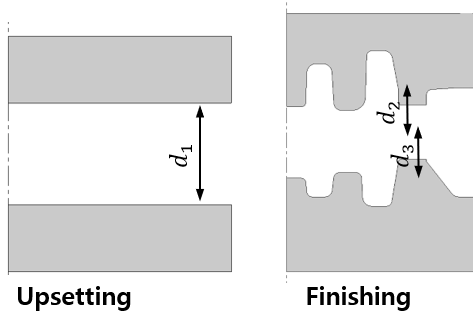
(a) Initial design (b) Discontinuity of grain flow lines
Figure 15.21 Pulley hot forging process and definition of design variables
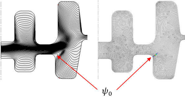
Figure 15.22 Local caving defect of the initial design and the objective function
There is a characteristic that the direction of the grain flow line density changes gradually. As characteristics of local-caving grain flow lines, one can cite the point that the \(x\)-axis and \(y\)-axis grain flow lines simultaneously undergo abrupt change and the point that the grain flow line density is relatively small in both directions. Based on these characteristics and consideration of the quantification indices of grain flow lines, it was confirmed by a trial-and-error method that the following function is effective in preventing such local-caving defects.
The design variables are defined in Figure 15.21, and the design variables that minimize the objective function of Equation (15.7) were determined. Figure 15.23 compares the grain flow lines of the initial design and the optimal design. As seen in this figure, by the optimization the parting line of the die where the flash occurs was lowered, and it can be seen that the change of the grain flow lines is extreme. Of course, the local caving defect of the initial design disappeared.
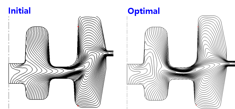
Figure 15.23 Comparison of the initial design and the optimal design