10 Structural Analysis of Dies

10.1 Definition and Formulation of the Die Structural Analysis Problem

The elasticity-mechanics problem is conceptually illustrated in Figure 10.1.

Figure 10.1 Conceptual diagram of the elasticity-mechanics problem

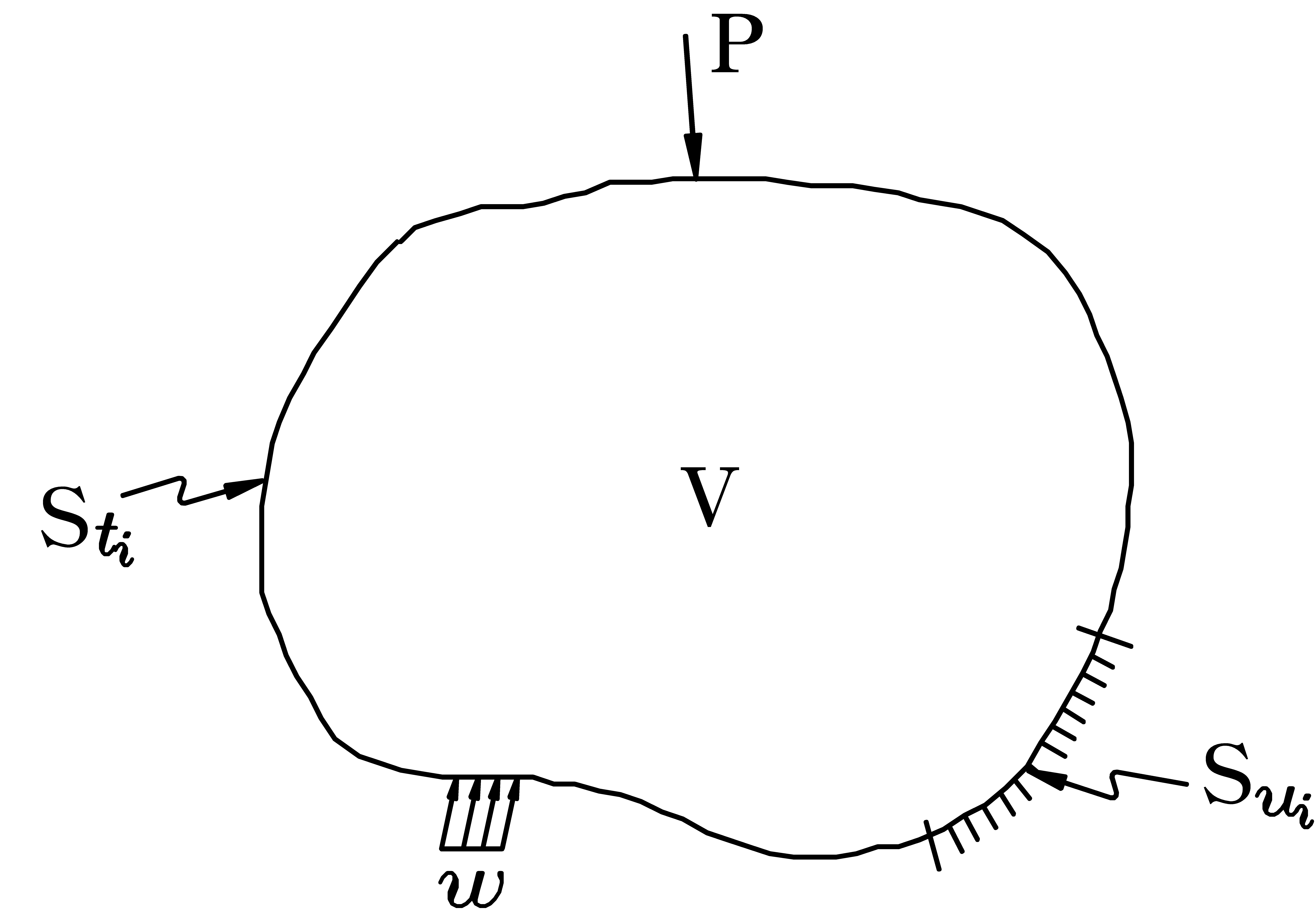
Structural analysis of a die is the process of finding the displacement field \(u_i\) that satisfies the geometric boundary conditions and the mechanical boundary conditions, and the various mechanical quantities, including the stress, derived from it. The die structural analysis problem consists of the analysis domain \(V\), the traction-prescribed boundary \(S_{t_i}\) where the traction is prescribed as \(\sigma_{ij}n_j = \bar{t}_i^{(n)}\), the displacement-prescribed boundary \(S_{u_i}\) where the displacement is prescribed as \(u_i = \bar{u}_i\), the contact surface \(S_c\) between the two bodies, and so on.

The two bodies, that is, the two die components, share a normal vector at the contact surface, and the contact surface is defined by the same normal vector \(n_i\). When the normal vector \(n_i\) is outward from a body, the contact boundary of that body is defined as \(S_c^+\), and conversely the contact boundary that is inward is denoted \(S_c^-\). That is, since the same normal vector is used at the contact boundary, \(S_c^+\) and \(S_c^-\) always exist at the contact boundary. \(S_c\) is used to represent both \(S_c^+\) and \(S_c^-\). The mechanical and geometric boundary conditions on \(S_c\) of the contact part between the two bodies are as follows. In the normal direction of the contact boundary,

\[u_n^{+c} = u_n^{-c} \quad \text{if} \quad \sigma_n^{+c} < 0 \tag{10.1}\]

\[\sigma_n^{+c} = 0 \quad \text{if} \quad u_n^{+c} - u_n^{-c} < 0 \tag{10.2}\]

and in the tangential direction,

\[\sigma_t^{+c} = -\sigma_t^{-c} = \mu |\sigma_n| \frac{(u_t^{-c} - u_t^{+c})}{|u_t^{-c} - u_t^{+c}|} \quad \text{if} \quad u_t^{-c} \neq u_t^{+c} \tag{10.3}\]

\[u_t^{-c} = u_t^{+c} \quad \text{if} \quad |\sigma_t| < \mu |\sigma_n| \tag{10.4}\]

Here the subscripts \(n\) and \(t\) denote the normal component and the tangential component, respectively, and the superscripts \(+c\) and \(-c\) denote the components on \(S_c^+\) and \(S_c^-\), respectively.

Equation (10.3) implies that when slip occurs at the contact surface, a friction stress acts in the direction opposing the slip according to the Coulomb friction law. When slip does not occur, the tangential boundary condition is governed by Equation (10.4), that is, it is regarded as part of the essential boundary conditions, and the magnitude of the friction stress at that time becomes smaller than \(\mu |\sigma_n|\). Using the penalty method, the condition of Equation (10.1) can be embedded in the principle of virtual work as shown in the following equation.

\[ \begin{aligned} \int_V \sigma_{ij} \delta\varepsilon_{ij} dV - \int_V f_i \delta u_i dV - \sum \int_{S_{t_i}} \bar{t}_i^{(n)} \delta u_i dS \\ + \int_{S_c} \beta (u_n^{+c} - u_n^{-c})(\delta u_n^{+c} - \delta u_n^{-c}) dS - \int_{S_c} \sigma_t \delta u_t dS = 0 \end{aligned} \tag{10.29} \]

Here \(S_{c'} (\subset S_c)\) denotes the mechanical contact boundary where \(\sigma_n^{+c} < 0\), and it is itself an unknown. This expression implies that, even if the boundary is geometrically attached, it becomes a free surface if no pressure acts on it. That is, \(S_c\) denotes the geometric contact boundary. The penalty constant \(\beta\) is a very large positive constant and has the physical meaning \(\sigma_n^{+c} = -\beta(u_n^{+c} - u_n^{-c})\).

The stress–strain relation is expressed as follows.

\[\sigma_{ij} = 2\mu\varepsilon_{ij} + \lambda\varepsilon_{kk} - (3\lambda + 2\mu)\alpha\Delta T\delta_{ij} \tag{10.30}\]

Here \(\mu\) and \(\lambda\) are the Lamé constants, and they have the following relations with the elastic modulus \(E\) and Poisson's ratio \(\nu\).

\[\mu = E / 2(1+\nu) \tag{10.31}\]

\[\lambda = \nu E / (1+\nu)(1-2\nu) \tag{10.32}\]

And \(\alpha\) is the coefficient of thermal expansion, and \(\Delta T\) denotes the difference between the current temperature and the reference temperature corresponding to the amount of shrink fit, that is, the thermal load.

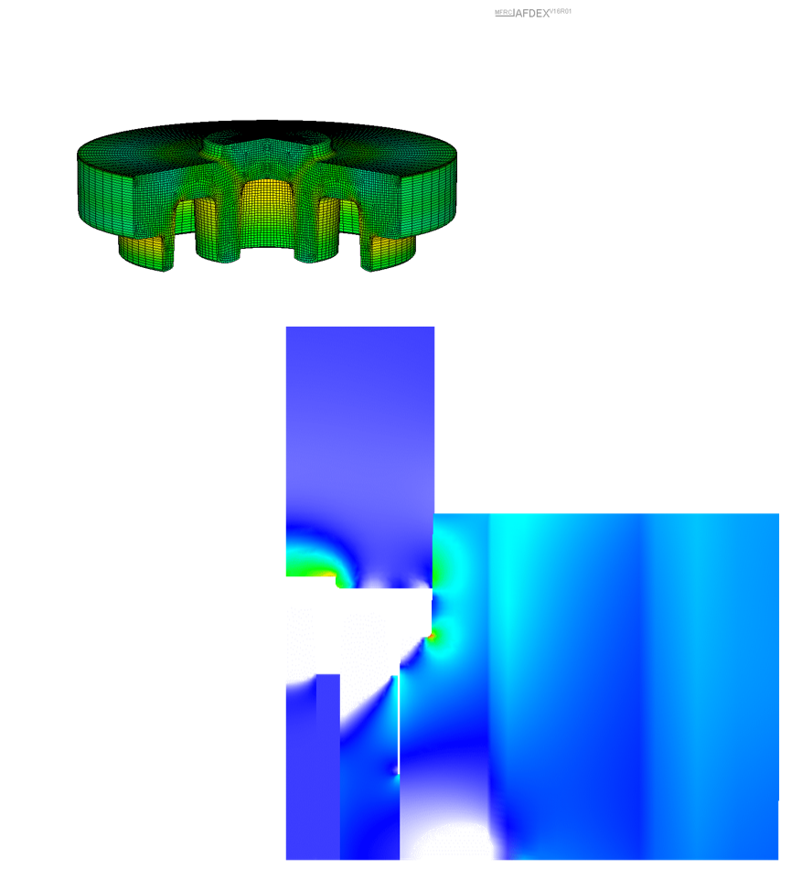
Figure 10.2 shows the die structural analysis results for a cold forging process and a hypothetical die design. In cold forging, a die-splitting technique is applied to prevent frequent fracture caused by stress concentration at the corners of the die. This example represents an extreme case of structural analysis of a split die.

(a) Two-dimensional

(b) Three-dimensional

Figure 10.2 Structural analysis of a hypothetical split die

10.2 Complete Simulation

In the analysis of bulk metal-forming processes such as forging, the deformation of the die itself is often not important. And analysis that considers the elastic deformation of the die, that is, complete simulation, has technical difficulties, so until recently it remained at the academic level. For this reason, most bulk metal-forming simulations have regarded the die as a rigid body.

With the recent advancement of bulk metal-forming simulation technology, the practical use of complete simulation technology is being realized. Complete simulation technology regards the die as an elastic body or an elasto-plastic body and performs a metal-forming simulation on the actual die shape, taking into account the elastic deformation of the die. However, the finite element method basically applies deformation to a workpiece that is more constrained than in reality, so its reaction force is inevitably larger than in reality. In some cases, the prediction may be 20–30% larger. Therefore, owing to the excessive change of the die caused by the overload, the range of variation of the analysis results can be larger than that of the solution obtained under the rigid-body assumption.

An example of complete simulation is shown in Figure 10.3. This example is an axisymmetric cold forging process in which the shrinkage and preload of the die due to shrink fitting are considered, and during the process analysis, the elastic deformation of the die due to the forming load and the shrink fit was considered. In other words, the effect of the die deformation caused by the elastic deformation of the die on the workpiece is reflected. An elasto-plastic finite element method capable of reflecting the elastic deformation of the material was used. Therefore, from a mechanical viewpoint, the assumptions were minimized. Such analysis of a metal-forming process is called complete simulation.

Figure 10.3 Example of complete simulation of an axisymmetric process

And the commonalities and differences between complete simulation and general analysis are detailed in Section 11.9.3 through the analysis of a scroll forging process.