3 Deformation of Solids

3.1 Displacement and Deformation

Newton regarded an object as a collection of material points. In general, an actual object consists of crystals and grain boundaries, and a crystal consists of a regular arrangement of atoms. Therefore, Newton's hypothesis closely resembles an actual object when viewed from a macroscopic point of view. For the investigation of mechanics problems from a macroscopic point of view, an object is regarded as a continuous collection of countless material points. This is called a continuum.

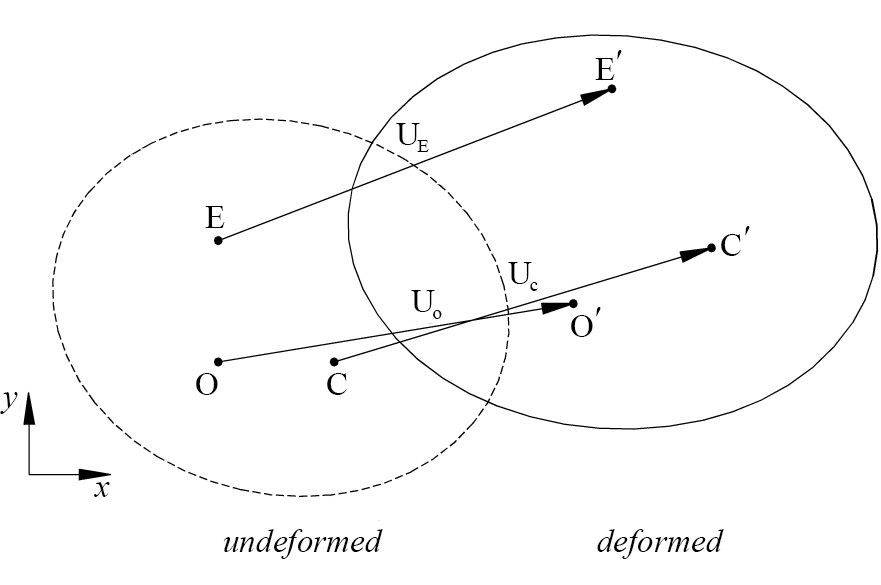
The displacement of a continuum, as shown in Figure 3.1, quantifies the change in position of a solid. The displacement generally differs at each material point or arbitrary point. Therefore, each component of the displacement vector \(u\) is a function of position, and since position is expressed by coordinates, displacement is a function of the coordinates. Of course, the displacement in a system to which a dynamic load is applied is also a function of time. The displacement that an object can undergo varies with the applied force. Since the combinations of forces that can be applied are infinite in number, the number of displacements that the object can experience is also infinite. Such a collection of displacements is called the displacement vector field or displacement field.

Displacement is divided into deformation and rigid body motion. That in which the distance between material points does not change despite the occurrence of displacement is called rigid body motion. The meaning of rigid body motion is clear. Therefore, deformation, which has the dictionary meaning of a change in shape, mathematically or mechanically means displacement with rigid body motion excluded.

In elasticity, plasticity, vibration theory, etc., deformation is emphasized, whereas in rigid body dynamics, deformation is neglected. In deformable body dynamics, both are emphasized. In elasticity and plasticity, the overall rigid body motion of an object is generally absent, but rigid body motion does occur partially. In dynamics, since the displacement due to rigid body motion is much larger than the displacement due to deformation, deformation is often neglected.

The displacement of a single material point is expressed by a vector, whereas the displacement of a solid, that is, the displacement field, is expressed by a vector function whose components are real functions. The method of formulating a solid mechanics problem by regarding the displacement field as the final unknown function is called the displacement method. Most mechanics problems are solved by the displacement method. Therefore, in the displacement method, a mechanics problem is the mathematical problem of finding, from the displacement field, the displacement that satisfies the equilibrium or equation of motion and the constitutive equations studied in Chapter 4. That displacement is mostly unique, and it is not unique in special problems such as the resonance phenomenon in vibration theory, the necking phenomenon in a tension test, and the buckling phenomenon in compressive deformation.

Figure 3.1 Visualization of the displacement field

3.2 Deformation Gradient Tensor

Figure 3.2 conceptualizes the deformation of an object. That is, it expresses Figure 3.1 from a different angle. State A represents the shape of the initial, undeformed state, and state B represents the deformed state. The deformation of a general object occurs as a combination of (1) translation, (2) rigid body rotation, and (3) pure stretch of the object.

In the figure, the deformation of the object is measured in the \(XYZ\) coordinate system. Consider that an infinitesimal line segment \(PQ\), that is, the vector \(d\mathbf{X}\), is embedded in the object in state A. In state A, the position of point \(P\) is represented by the vector \(\mathbf{X}\). Point \(P\) moves by the vector \(\mathbf{u}\) from state A to point \(P'\) in state B. Point \(P'\) is represented by the vector \(\mathbf{x}\) and can be expressed by the following equation.

\[\mathbf{x} = \mathbf{X} + \mathbf{u} \tag{3.1}\]

Figure 3.2 Deformation of an object from the initial undeformed state to the current deformed state

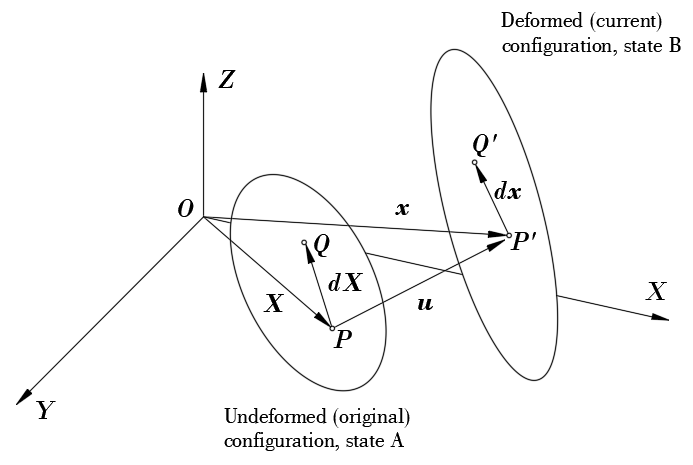
The infinitesimal line segment \(PQ\) in state A, that is, the vector \(d\mathbf{X}\), deforms into \(P'Q'\) in state B, that is, the vector \(d\mathbf{x}\). In this case, the relationship between the two vectors can be expressed by the following equation using the deformation gradient \(\mathbf{F}\).

\[d\mathbf{x}=\mathbf{F}d\mathbf{X}\tag{3.2}\]

or

\[d\mathbf{x}=\frac{\partial \mathbf{x}}{\partial \mathbf{X}}d\mathbf{X}\tag{3.3}\]

Expressed in terms of vector and matrix components, it is as in the following equation.

\[\begin{bmatrix} dx \\ dy \\ dz \end{bmatrix} = \begin{bmatrix} \frac{\partial x}{\partial X} & \frac{\partial x}{\partial Y} & \frac{\partial x}{\partial Z} \\ \frac{\partial y}{\partial X} & \frac{\partial y}{\partial Y} & \frac{\partial y}{\partial Z} \\ \frac{\partial z}{\partial X} & \frac{\partial z}{\partial Y} & \frac{\partial z}{\partial Z} \end{bmatrix} \begin{bmatrix} dX \\ dY \\ dZ \end{bmatrix}\tag{3.4}\]

That is,

\[\mathbf{F}=\frac{\partial \mathbf{x}}{\partial \mathbf{X}}\tag{3.5}\]

holds. The deformation gradient tensor \(\mathbf{F}\) completely includes, among the deformations, the rigid body rotation and pure stretch excluding translation. Since rigid body rotation does not cause deformation of the object, only the pure stretch component causes deformation of the object. Therefore, the process of separating the rigid body rotation and pure stretch from the deformation gradient \(\mathbf{F}\) is necessary for the deformation analysis of the object.

3.3 Strain

Let us quantify the deformation of an object. Displacement consists of translation, rigid body motion, and pure stretch. In an object undergoing pure rigid body motion, no deformation occurs, and the length between all material points does not change. Therefore, the change in length between material points can be used as a measure to quantify the deformation of an object. In this section, we study strain, which was introduced to quantitatively express the deformation at an arbitrary point.

Under the assumption that a solid is undergoing small deformation, let us examine the calculation of the small strain tensor.

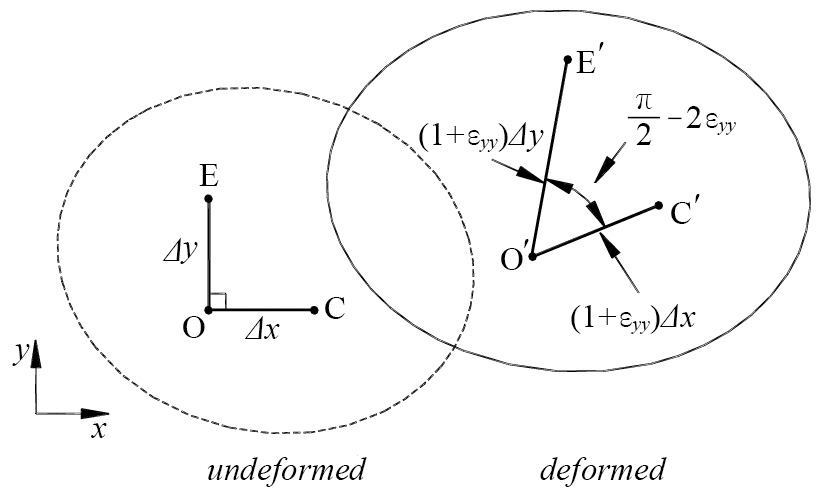
Let us quantify the deformation at point \(O\) on the two-dimensional plane in Figure 3.3 (the quantification of one-dimensional deformation is replaced by the content on the tension test in Chapter 4). The deformation at this point is quantified by the change in length per unit length of the line segments \(OC\) and \(OE\), which are adjacent to point \(O\) and parallel to the \(x\)-axis and \(y\)-axis, respectively, and by the change in the angle \(\angle EOC\). The rate of change in length of the line segment \(OC\) in the \(x\)-direction, that is, the change in length per unit length, is defined as

\[\lim_{C \to O}(\overline{O'C'} - \overline{OC}) / \overline{OC} \equiv \varepsilon_{xx}\tag{3.6}\]

and the amount of decrease in the angle between the \(x\)-axis and \(y\)-axis is defined as follows.

\[\lim_{C, E \to O}(\angle EOC - \angle E'O'C') \equiv 2\varepsilon_{xy}\tag{3.7}\]

The other strain components \(\varepsilon_{yy}\), \(\varepsilon_{zz}\), \(\varepsilon_{yz}\), \(\varepsilon_{zx}\), \(\varepsilon_{zy}\), \(\varepsilon_{xz}\), etc., are defined in the same way. The strain at a point in three-dimensional space is expressed in the following matrix form.

\[\varepsilon_{ij}, \quad [\varepsilon_{ij}] = \begin{bmatrix} \varepsilon_{11} & \varepsilon_{12} & \varepsilon_{13} \\ \varepsilon_{21} & \varepsilon_{22} & \varepsilon_{23} \\ \varepsilon_{31} & \varepsilon_{32} & \varepsilon_{33} \end{bmatrix} = \begin{bmatrix} \varepsilon_{xx} & \varepsilon_{xy} & \varepsilon_{xz} \\ \varepsilon_{yx} & \varepsilon_{yy} & \varepsilon_{yz} \\ \varepsilon_{zx} & \varepsilon_{zy} & \varepsilon_{zz} \end{bmatrix}\tag{3.8}\]

Here, \(\varepsilon_{ii}\) (the summation convention with respect to \(i\) is not followed) denotes the change in length per unit length of a line segment in the \(x_i\)-axis direction, and is the normal strain. \(\varepsilon_{ij}\) (\(i \neq j\)) denotes one half of the change in angle between line segment elements in the orthogonal \(x_i\)-axis direction and \(x_j\)-axis direction, and is the shear strain. A positive normal strain means that the length of the line segment has increased, and a positive shear strain means that the angle \(\angle EOC\) has decreased.

Figure 3.3 Quantification of the deformation of a solid

Using the \(x-y-z\) rectangular coordinate system, the relationship between the strain (\(\varepsilon_{xx}, \varepsilon_{yy}, \varepsilon_{zz}, \varepsilon_{xy}, \varepsilon_{yz}, \varepsilon_{zx}\)) at a point of a three-dimensional object and the displacement field \(\mathbf{u} = [u_x, u_y, u_z]^\text{T}\) is as follows.

\[ \varepsilon_{ij} = \frac{1}{2} \left( \frac{\partial u_i}{\partial x_j} + \frac{\partial u_j}{\partial x_i} \right) \quad \text{or} \quad \begin{aligned} \varepsilon_{xx} &= \frac{\partial u_x}{\partial x} \\ \varepsilon_{yy} &= \frac{\partial u_y}{\partial y} \\ \varepsilon_{zz} &= \frac{\partial u_z}{\partial z} \\ \varepsilon_{xy} &= \frac{1}{2} \left( \frac{\partial u_x}{\partial y} + \frac{\partial u_y}{\partial x} \right) \\ \varepsilon_{yz} &= \frac{1}{2} \left( \frac{\partial u_y}{\partial z} + \frac{\partial u_z}{\partial y} \right) \\ \varepsilon_{zx} &= \frac{1}{2} \left( \frac{\partial u_z}{\partial x} + \frac{\partial u_x}{\partial z} \right) \end{aligned} \tag{3.9} \]

From Eq. (3.9), it can be seen that the strain satisfies \(\varepsilon_{ij} = \varepsilon_{ji}\). Often, when \(i \neq j\), one sets \(\gamma_{ij} = 2\varepsilon_{ij}\) and calls \(\gamma_{ij}\) the engineering shear strain. What must be kept in mind here is that \(\gamma_{ij}\) is not a second-order tensor quantity. Since strain is a second-order tensor, it follows the following transformation law.

\[ \varepsilon'_{ij} = \sum_{p=1}^{3} \sum_{q=1}^{3} T_{ip} T_{jq} \varepsilon_{pq} \]

or

\[ \begin{pmatrix} \varepsilon_{1'1'} & \varepsilon_{1'2'} & \varepsilon_{1'3'} \\ \varepsilon_{2'1'} & \varepsilon_{2'2'} & \varepsilon_{2'3'} \\ \varepsilon_{3'1'} & \varepsilon_{3'2'} & \varepsilon_{3'3'} \end{pmatrix} = \begin{pmatrix} T_{1'1} & T_{1'2} & T_{1'3} \\ T_{2'1} & T_{2'2} & T_{2'3} \\ T_{3'1} & T_{3'2} & T_{3'3} \end{pmatrix} \begin{pmatrix} \varepsilon_{11} & \varepsilon_{12} & \varepsilon_{13} \\ \varepsilon_{21} & \varepsilon_{22} & \varepsilon_{23} \\ \varepsilon_{31} & \varepsilon_{32} & \varepsilon_{33} \end{pmatrix} \begin{pmatrix} T_{1'1} & T_{2'1} & T_{3'1} \\ T_{1'2} & T_{2'2} & T_{3'2} \\ T_{1'3} & T_{2'3} & T_{3'3} \end{pmatrix} \tag{3.10} \]

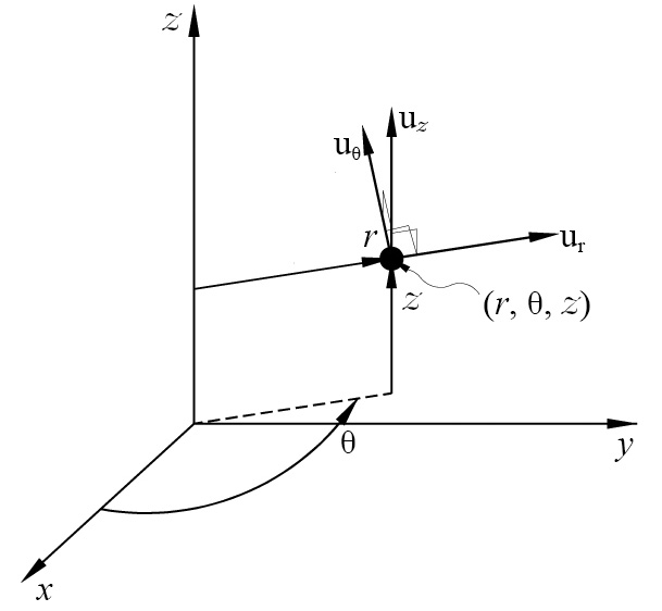
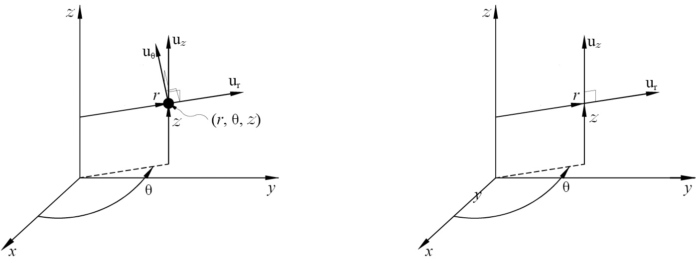
As shown in Figure 3.4, in the \(r-\theta-z\) cylindrical coordinate system, the relationship between the strain (\(\varepsilon_{rr}, \varepsilon_{\theta\theta}, \varepsilon_{zz}, \varepsilon_{r\theta}, \varepsilon_{\theta z}, \varepsilon_{zr}\)) and the displacement \(\mathbf{u} = [u_r, u_\theta, u_z]^\text{T}\) is as follows.

\[ \begin{aligned} \varepsilon_{rr} &= \frac{\partial u_r}{\partial r} \\ \varepsilon_{\theta\theta} &= \frac{1}{r} \frac{\partial u_\theta}{\partial \theta} + \frac{u_r}{r} \\ \varepsilon_{zz} &= \frac{\partial u_z}{\partial z} \\ \varepsilon_{r\theta} &= \frac{1}{2} \left( \frac{1}{r} \frac{\partial u_r}{\partial \theta} + \frac{\partial u_\theta}{\partial r} - \frac{u_\theta}{r} \right) \\ \varepsilon_{\theta z} &= \frac{1}{2} \left( \frac{\partial u_\theta}{\partial z} + \frac{1}{r} \frac{\partial u_z}{\partial \theta} \right) \\ \varepsilon_{zr} &= \frac{1}{2} \left( \frac{\partial u_z}{\partial r} + \frac{\partial u_r}{\partial z} \right) \end{aligned} \tag{3.11} \]

Figure 3.4 Displacement in the cylindrical coordinate system

So far, the small strain has been derived from the geometric meaning of deformation. The small strain tensor obtained in this way has the advantage of an easy calculation process, but it has the problem of accompanying errors in the case of large deformation because it includes translation and rigid body motion.

Now let us examine the method of accurately calculating the strain in the case where an object is undergoing general large deformation. Using the deformation gradient tensor defined in Section 3.2, the strain can be mathematically defined from the pure stretch component excluding translation and rigid body motion. In Figure 3.2, the length \(ds\) of the infinitesimal line segment \(P'Q'\) in state B can be expressed as in the following equation.

\[ \begin{aligned} ds^2 &= d\mathbf{x} \cdot d\mathbf{x} = (\mathbf{F}d\mathbf{X}) \cdot (\mathbf{F}d\mathbf{X}) = d\mathbf{X}^\text{T}\mathbf{F}^\text{T}\mathbf{F}d\mathbf{X} \\ &= d\mathbf{X} \left( \frac{\partial \mathbf{x}}{\partial \mathbf{X}} \right)^\text{T} \frac{\partial \mathbf{x}}{\partial \mathbf{X}} d\mathbf{X} = d\mathbf{X}\mathbf{C}d\mathbf{X} \end{aligned} \tag{3.12} \]

Here,

\[ \mathbf{C} = \mathbf{F}^\text{T}\mathbf{F} \tag{3.13} \]

and \(\mathbf{C}\) is the Cauchy-Green tensor.

On the other hand, the length \(dS\) of the initial infinitesimal line segment \(PQ\) can be expressed as follows.

\[ dS^2 = d\mathbf{X}^\text{T}d\mathbf{X} \tag{3.14} \]

Since the lengths \(ds\) and \(dS\) of the infinitesimal line segments are pure changes in length independent of translation and rigid body rotation, they provide a suitable basis for obtaining the strain due to pure stretch. Using the fact that the difference of the squares of the infinitesimal lengths is constant regardless of translation and rigid body rotation, the following equation is derived.

\[ \begin{aligned} ds^2 - dS^2 &= d\mathbf{x}^\text{T}d\mathbf{x} - d\mathbf{X}^\text{T}d\mathbf{X} = (\mathbf{F}d\mathbf{X})^\text{T}(\mathbf{F}d\mathbf{X}) - d\mathbf{X}^\text{T}d\mathbf{X} \\ &= d\mathbf{X}^\text{T}\mathbf{F}^\text{T}\mathbf{F}d\mathbf{X} - d\mathbf{X}^\text{T}d\mathbf{X} = d\mathbf{X}^\text{T}(\mathbf{C} - \mathbf{I})d\mathbf{X} \end{aligned} \tag{3.15} \]

Here,

\[ \mathbf{E} = \frac{1}{2}(\mathbf{C} - \mathbf{I}) = \frac{1}{2}(\mathbf{F}^\text{T}\mathbf{F} - \mathbf{I}) \tag{3.16} \]

and \(\mathbf{E}\) is the Green-Lagrange strain tensor, which provides a strain independent of translation and rigid body rotation. On the other hand, from Eqs. (3.1) and (3.5), the following equation is obtained.

\[ \mathbf{F} = \frac{\partial \mathbf{x}}{\partial \mathbf{X}} = \frac{\partial (\mathbf{u} + \mathbf{X})}{\partial \mathbf{X}} = \frac{\partial \mathbf{u}}{\partial \mathbf{X}} + \mathbf{I} \tag{3.17} \]

Substituting Eq. (3.17) into (3.16) gives the following.

\[ \begin{aligned} \mathbf{E} &= \frac{1}{2}(\mathbf{F}^\text{T}\mathbf{F} - \mathbf{I}) = \frac{1}{2} \left[ \left[ \frac{\partial \mathbf{u}}{\partial \mathbf{X}} + \mathbf{I} \right]^\text{T} \left[ \frac{\partial \mathbf{u}}{\partial \mathbf{X}} + \mathbf{I} \right] - \mathbf{I} \right] \\ &= \frac{1}{2} \left[ \frac{\partial \mathbf{u}}{\partial \mathbf{X}} + \left( \frac{\partial \mathbf{u}}{\partial \mathbf{X}} \right)^\text{T} + \left( \frac{\partial \mathbf{u}}{\partial \mathbf{X}} \right)^\text{T} \frac{\partial \mathbf{u}}{\partial \mathbf{X}} \right] \end{aligned} \tag{3.18} \]

Omitting the second-order term in Eq. (3.18) gives the small strain tensor of Eq. (3.19).

\[ \mathbf{E} = \frac{1}{2} \left[ \frac{\partial \mathbf{u}}{\partial \mathbf{X}} + \left( \frac{\partial \mathbf{u}}{\partial \mathbf{X}} \right)^\text{T} \right] \tag{3.19} \]

That is, Eq. (3.19) is an approximate form of the Green-Lagrange strain that is independent of translation and rigid body motion, and it can be seen that it is not independent of translation and rigid body motion.

Since the Green-Lagrange strain tensor is based on the difference of the squares of lengths, in the case of large deformation, a large difference from the true strain occurs. Therefore, a method of obtaining the true strain is needed. Using the polar decomposition theorem [3.1], the deformation gradient tensor \(\mathbf{F}\) is expressed as the product of the rotation tensor \(\mathbf{R}\) and the right stretch tensor \(\mathbf{U}\), as in the following equation.

\[ \mathbf{F} = \mathbf{RU} \tag{3.20} \]

Here, \(\mathbf{R}\) is an orthogonal (\(\mathbf{R}^\text{T}\mathbf{R} = \mathbf{I}\)) rotation tensor, and \(\mathbf{U}\) is a symmetric stretch tensor representing pure stretch.

The relationship between the Cauchy-Green tensor \(\mathbf{C}\) and the right stretch tensor \(\mathbf{U}\) can be expressed by the following equation.

\[ \mathbf{C} = \mathbf{F}^\text{T}\mathbf{F} = (\mathbf{RU})^\text{T}\mathbf{RU} = \mathbf{U}^\text{T}\mathbf{R}^\text{T}\mathbf{RU} = \mathbf{U}^\text{T}\mathbf{U} = \mathbf{U}^2 \tag{3.21} \]

Using Eq. (3.21) and the properties of the stretch tensor, the true strain can be obtained as follows.

\[ \pmb{\varepsilon} = \ln \mathbf{U} = \frac{1}{2} \ln \mathbf{C} \tag{3.22} \]

The true strain \(\pmb{\varepsilon}\) obtained in this way is independent of rigid body rotation and depends only on the stretch of the object, and is therefore suitable for deformation analysis.

3.4 Velocity Field and Strain Rate

The displacement field is a function of position and time. By differentiating the displacement field with respect to time, the velocity field can be obtained as follows.

\[ \mathbf{v} = \frac{d\mathbf{u}}{dt}, \quad v_i = \frac{du_i}{dt} \quad \text{or} \quad v_i = \dot{u}_i \tag{3.23} \]

Here, assume that a displacement occurred over \(\Delta t\) due to the velocity field \(v_i\). However, it is assumed that \(\Delta t\) is sufficiently small that the change in velocity during this time can be neglected and that it causes a sufficiently small deformation. Then, since \(u_i = v_i \Delta t\), the strain increments \(\Delta \varepsilon_{ij}\) and \(d\varepsilon_{ij}\) that accumulated during this time are, respectively, as follows.

\[ \begin{aligned} \Delta \varepsilon_{ij} &= \frac{1}{2} \left( \frac{\partial (v_i \Delta t)}{\partial x_j} + \frac{\partial (v_j \Delta t)}{\partial x_i} \right) = \frac{1}{2} \left( \frac{\partial v_i}{\partial x_j} + \frac{\partial v_j}{\partial x_i} \right) \Delta t \\ d\varepsilon_{ij} &= \frac{1}{2} \left( \frac{\partial v_i}{\partial x_j} + \frac{\partial v_j}{\partial x_i} \right) dt \end{aligned} \tag{3.24} \]

On the other hand, the symmetric part of the velocity gradient tensor \(\frac{\partial v_i}{\partial x_j}\),

\[ \dot{\varepsilon}_{ij} \equiv \frac{1}{2} \left( \frac{\partial v_i}{\partial x_j} + \frac{\partial v_j}{\partial x_i} \right) \tag{3.25} \]

is called the strain rate. The strain rate belongs to the second-order tensor quantities. The time parameter \(t\) denotes a virtual time, and in some cases it may be regarded as the actual time. For instance, in the analysis of a plastic forming process assumed to have no velocity effect, if the actual process velocity is not input, \(t\) is a virtual time, and when solving a viscoplastic problem, since velocity affects the process, \(t\) has the meaning of the actual time.

In general, \(\varepsilon_{ij} \neq \int_0^t \dot{\varepsilon}_{ij} dt\). This is because the principal strain axes change together with the occurrence of the displacement field.

3.5 Principal Strain, Principal Strain Rate, and Invariants

Strain and strain rate are second-order tensor quantities. Therefore, as with the stress tensor, from the following eigenvalue problems for the strain tensor \(\varepsilon_{ij}\) and the strain rate tensor \(\dot{\varepsilon}_{ij}\),

\[ \sum_{j=1}^{3} \varepsilon_{ij}n_j = \varepsilon n_i \quad \text{or} \quad \begin{bmatrix} \varepsilon_{xx} & \varepsilon_{xy} & \varepsilon_{xz} \\ \varepsilon_{yx} & \varepsilon_{yy} & \varepsilon_{yz} \\ \varepsilon_{zx} & \varepsilon_{zy} & \varepsilon_{zz} \end{bmatrix} \begin{bmatrix} n_x \\ n_y \\ n_z \end{bmatrix} = \varepsilon \begin{bmatrix} n_x \\ n_y \\ n_z \end{bmatrix} \tag{3.26} \]

\[ \sum_{j=1}^{3} \dot{\varepsilon}_{ij}n_j = \dot{\varepsilon} n_i \quad \text{or} \quad \begin{bmatrix} \dot{\varepsilon}_{xx} & \dot{\varepsilon}_{xy} & \dot{\varepsilon}_{xz} \\ \dot{\varepsilon}_{yx} & \dot{\varepsilon}_{yy} & \dot{\varepsilon}_{yz} \\ \dot{\varepsilon}_{zx} & \dot{\varepsilon}_{zy} & \dot{\varepsilon}_{zz} \end{bmatrix} \begin{bmatrix} n_x \\ n_y \\ n_z \end{bmatrix} = \dot{\varepsilon} \begin{bmatrix} n_x \\ n_y \\ n_z \end{bmatrix} \tag{3.27} \]

the three principal strains \(\varepsilon = \varepsilon_1, \varepsilon_2, \varepsilon_3\) and principal strain rates \(\dot{\varepsilon} = \dot{\varepsilon}_1, \dot{\varepsilon}_2, \dot{\varepsilon}_3\) are defined. Since strain and strain rate are second-order tensor quantities, the following invariants are defined.

\[ L_1 = \sum_{i=1}^{3} \varepsilon_{ii} = \varepsilon_{xx} + \varepsilon_{yy} + \varepsilon_{zz} \tag{3.28} \]

\[ L_2 = \frac{1}{2} \sum_{i=1}^{3} \sum_{j=1}^{3} (\varepsilon_{ij}\varepsilon_{ji} - \varepsilon_{ii}\varepsilon_{jj}) = -\varepsilon_{xx}\varepsilon_{yy} - \varepsilon_{yy}\varepsilon_{zz} - \varepsilon_{zz}\varepsilon_{xx} + \varepsilon_{xy}^2 + \varepsilon_{yz}^2 + \varepsilon_{zx}^2 \tag{3.29} \]

\[ L_3 = |\varepsilon_{ij}| = \varepsilon_{xx}\varepsilon_{yy}\varepsilon_{zz} + 2\varepsilon_{xy}\varepsilon_{yz}\varepsilon_{zx} - \varepsilon_{xx}\varepsilon_{yz}^2 - \varepsilon_{yy}\varepsilon_{zx}^2 - \varepsilon_{zz}\varepsilon_{xy}^2 \tag{3.30} \]

\[ \dot{L}_1 = \sum_{i=1}^{3} \dot{\varepsilon}_{ii} = \dot{\varepsilon}_{xx} + \dot{\varepsilon}_{yy} + \dot{\varepsilon}_{zz} \tag{3.31} \]

\[ \dot{L}_2 = \frac{1}{2} \sum_{i=1}^{3} \sum_{j=1}^{3} (\dot{\varepsilon}_{ij}\dot{\varepsilon}_{ji} - \dot{\varepsilon}_{ii}\dot{\varepsilon}_{jj}) = -\dot{\varepsilon}_{xx}\dot{\varepsilon}_{yy} - \dot{\varepsilon}_{yy}\dot{\varepsilon}_{zz} - \dot{\varepsilon}_{zz}\dot{\varepsilon}_{xx} + \dot{\varepsilon}_{xy}^2 + \dot{\varepsilon}_{yz}^2 + \dot{\varepsilon}_{zx}^2 \tag{3.32} \]

\[ \dot{L}_3 = |\dot{\varepsilon}_{ij}| = \dot{\varepsilon}_{xx}\dot{\varepsilon}_{yy}\dot{\varepsilon}_{zz} + 2\dot{\varepsilon}_{xy}\dot{\varepsilon}_{yz}\dot{\varepsilon}_{zx} - \dot{\varepsilon}_{xx}\dot{\varepsilon}_{yz}^2 - \dot{\varepsilon}_{yy}\dot{\varepsilon}_{zx}^2 - \dot{\varepsilon}_{zz}\dot{\varepsilon}_{xy}^2 \tag{3.33} \]

Here, the physical meanings of \(L_1\) and \(\dot{L}_1\) are the volumetric change rate and the rate of the volumetric change rate, respectively. If the material is incompressible, this value must be zero. Therefore, the incompressibility condition is expressed by the following equation.

\[ L_1 = \sum_{i=1}^{3} \varepsilon_{ii} = 0, \quad \dot{L}_1 = \sum_{i=1}^{3} \dot{\varepsilon}_{ii} = 0 \tag{3.34} \]

The effective strain \(\bar{\varepsilon}\) and the effective strain rate \(\dot{\bar{\varepsilon}}\) are defined as follows.

\[ \bar{\varepsilon} = \sqrt{\frac{2}{3} \sum_{i=1}^{3} \sum_{j=1}^{3} \varepsilon'_{ij}\varepsilon'_{ij}} = \frac{\sqrt{2}}{3} \left[ (\varepsilon_{xx} - \varepsilon_{yy})^2 + (\varepsilon_{yy} - \varepsilon_{zz})^2 + (\varepsilon_{zz} - \varepsilon_{xx})^2 + 6(\varepsilon_{xy}^2 + \varepsilon_{yz}^2 + \varepsilon_{zx}^2) \right]^{\frac{1}{2}} \tag{3.35} \]

\[ \dot{\bar{\varepsilon}} = \sqrt{\frac{2}{3} \sum_{i=1}^{3} \sum_{j=1}^{3} \dot{\varepsilon}'_{ij}\dot{\varepsilon}'_{ij}} = \frac{\sqrt{2}}{3} \left[ (\dot{\varepsilon}_{xx} - \dot{\varepsilon}_{yy})^2 + (\dot{\varepsilon}_{yy} - \dot{\varepsilon}_{zz})^2 + (\dot{\varepsilon}_{zz} - \dot{\varepsilon}_{xx})^2 + 6(\dot{\varepsilon}_{xy}^2 + \dot{\varepsilon}_{yz}^2 + \dot{\varepsilon}_{zx}^2) \right]^{\frac{1}{2}} \tag{3.36} \]

3.6 Plane Strain Problems and Axisymmetric Problems

When the components of the strain tensor or strain rate tensor for a certain single direction are all zero, it is called plane strain. For convenience, let us assume that direction is the \(z(x_3)\)-axis direction. The displacement and velocity in plane strain are

\[ u_x = u_x(x, y), \quad u_y = u_y(x, y), \quad u_z = 0 \tag{3.37} \]

\[ v_x = v_x(x, y), \quad v_y = v_y(x, y), \quad v_z = 0 \tag{3.38} \]

and the strain and strain rate tensors are expressed in the following reduced form.

\[ [\varepsilon_{ij}] = \begin{bmatrix} \varepsilon_{xx} & \varepsilon_{xy} \\ \varepsilon_{yx} & \varepsilon_{yy} \end{bmatrix} = \begin{bmatrix} \varepsilon_{11} & \varepsilon_{12} \\ \varepsilon_{21} & \varepsilon_{22} \end{bmatrix} \tag{3.39} \]

\[ [\dot{\varepsilon}_{ij}] = \begin{bmatrix} \dot{\varepsilon}_{xx} & \dot{\varepsilon}_{xy} \\ \dot{\varepsilon}_{yx} & \dot{\varepsilon}_{yy} \end{bmatrix} = \begin{bmatrix} \dot{\varepsilon}_{11} & \dot{\varepsilon}_{12} \\ \dot{\varepsilon}_{21} & \dot{\varepsilon}_{22} \end{bmatrix} \tag{3.40} \]

Representative problems that belong to plane strain problems in engineering are dams and thin-plate rolling. In a dam, the displacement in the longitudinal direction is small compared with the direction in which the water flows. In thin-plate rolling, since the amount of width spread is small, the assumption of Eq. (3.38) is useful in engineering. Therefore, it belongs to plane strain problems. Two-dimensional analysis of plastic forming processes is mainly performed under the assumption of a plane strain problem. A plane strain problem is based on the assumption that no material flow occurs in the \(z(x_3)\)-axis direction.

Axisymmetric problems belong to particular problems even among three-dimensional problems. An axisymmetric problem must be geometrically axisymmetric, must also be axisymmetric in mechanical aspects such as loads and boundary conditions, and must also be axisymmetric in terms of material. As described above, although the conditions for axial symmetry are demanding, there are many problems that can be regarded as axisymmetric problems in engineering analysis. Axisymmetric problems are generally formulated in the \(r-\theta-z\) cylindrical coordinate system. Figure 3.5(a) defines the displacement vector \([u_r, u_\theta, u_z]^\text{T}\) in the cylindrical coordinate system. Under the axisymmetric condition, there is no displacement in the circumferential direction, and the other displacement components are also not functions of the circumferential coordinate \(\theta\). That is,

\[ u_r = u_r(r, z), \quad u_\theta = 0, \quad u_z = u_z(r, z) \tag{3.41} \]

holds. Therefore, the relationship between the non-zero strain components and the displacement is as follows.

\[ \begin{bmatrix} \varepsilon_{rr} \\ \varepsilon_{\theta\theta} \\ \varepsilon_{zz} \\ \varepsilon_{rz} \end{bmatrix} = \begin{bmatrix} \frac{\partial u_r}{\partial r} \\ \frac{u_r}{r} \\ \frac{\partial u_z}{\partial z} \\ \frac{1}{2}\left(\frac{\partial u_r}{\partial z} + \frac{\partial u_z}{\partial r}\right) \end{bmatrix} \tag{3.42} \]

Similarly, the relationship between the strain rate components and the velocity is as follows.

\[ \begin{bmatrix} \dot{\varepsilon}_{rr} \\ \dot{\varepsilon}_{\theta\theta} \\ \dot{\varepsilon}_{zz} \\ \dot{\varepsilon}_{rz} \end{bmatrix} = \begin{bmatrix} \frac{\partial v_r}{\partial r} \\ \frac{v_r}{r} \\ \frac{\partial v_z}{\partial z} \\ \frac{1}{2}\left(\frac{\partial v_r}{\partial z} + \frac{\partial v_z}{\partial r}\right) \end{bmatrix} \tag{3.43} \]

As shown in Figure 3.5(b), an axisymmetric problem is determined by the displacement fields \(u_r\) and \(u_z\) or the velocity fields \(v_r\) and \(v_z\). Therefore, although the analysis domain is a two-dimensional plane, in the actual computation the volume is automatically taken into account by the \(r\)-coordinate.

(a) Three-dimensional problem (b) Axisymmetric problem

Figure 3.5 Definition of the displacement vector in the cylindrical coordinate system and the axisymmetric problem

3.7 Idealization of the Strain Rate

The strain rate is divided into the quantity that is not recovered when the load is removed (\(\dot{\varepsilon}_{ij}^p\)) and the remaining quantity (\(\dot{\varepsilon}_{ij}^d\)). That is,

\[ \dot{\varepsilon}_{ij} = \dot{\varepsilon}_{ij}^p + \dot{\varepsilon}_{ij}^d \tag{3.44} \]

and \(\dot{\varepsilon}_{ij}^p\) and \(\dot{\varepsilon}_{ij}^d\) are called the plastic strain rate component and the difference strain rate component, respectively. The geometric meaning of the plastic strain rate component is clearly explained as unrecoverable deformation. On the other hand, the difference strain rate component is used in a somewhat comprehensive sense because it includes elements that are unclear from a macroscopic point of view, such as elasticity and creep. In most cases, the difference strain rate component is regarded as the elastic strain rate component or is neglected. In this case, for the former, that is,

\[ \dot{\varepsilon}_{ij}^d = \dot{\varepsilon}_{ij}^e \tag{3.45} \]

the case assuming this is called elastoplastic, and for the latter, that is,

\[ \dot{\varepsilon}_{ij}^d = 0 \tag{3.46} \]

the case assuming this is called rigid-plastic. Therefore, in rigid-plastic theory, \(\dot{\varepsilon}_{ij}\) and \(\dot{\bar{\varepsilon}}\) denote \(\dot{\varepsilon}_{ij}^p\) and \(\dot{\bar{\varepsilon}}^p\), respectively.