1 Introduction
Transparent materials possess countless paths through which light can pass. Metallic materials are opaque owing to the vibration of the outermost electrons and the motion of free electrons. Because of defects such as dislocations and atomic arrangements, as well as impurities, the behavioral characteristics at adjacent material points differ greatly, and the uncertainty is very high. From the microscopic viewpoint of atomic scale, a material is discontinuous and its behavioral characteristics vary with time. Such behavioral characteristics are effectively unusable without statistical treatment. From the viewpoint of the crystal scale, the situation improves considerably, but because of crystal boundaries, impurities, crystal orientation, and so on, it is impossible to obtain continuous and uniform behavioral characteristics of the material. For this reason, the results of engineering analysis based on the microscopic approach differ somewhat from actual macroscopic phenomena.
Once the region of interest exceeds a certain size, the behavioral characteristics of the material become statistically stable. Such behavioral characteristics are referred to as macroscopic behavioral characteristics. The macroscopic approach of mechanics focuses on identifying the macroscopic behavioral characteristics of a body. The macroscopic approach starts from the assumption that the material is a continuum. That is, the body subjected to engineering analysis is regarded as being composed of a set of continuous particles, in which adjacent particles are connected to one another to form a continuous body of a definite shape, and each particle is assumed to follow the macroscopic characteristics of the material. A continuum must maintain its continuity even after deformation. In other words, all particles of the body before and after deformation must have a one-to-one correspondence. Most bodies treated in engineering analysis can be regarded as continua from the macroscopic viewpoint. Solids, of course, also belong to continua.
Solid mechanics, including plasticity, is explained by the displacement method, viewed from the standpoint of displacement, and the force method, viewed from the standpoint of force. Figure 1.1 illuminates the continuum mechanics problem from the standpoint of the displacement method (in the figure, the subscript after a comma denotes partial differentiation with respect to the coordinate axis of that subscript, following the index notation used throughout all equations; see Appendix A). In the displacement method, displacement is regarded as the final unknown of continuum mechanics, and other mechanical quantities are treated as quantities derived from displacement. A continuum mechanics problem is largely composed of three elements: the governing equations, the constitutive equations, and the deformation-related equations. The governing equations deal with force equilibrium, the constitutive equations with the relationship between force and deformation, and the deformation-related equations with the geometry of deformation, that is, the relations of strain-displacement, strain rate-velocity, and so on. Since such equations are expressed as differential equations, they are accompanied by the boundary and initial conditions necessary to obtain a unique solution.
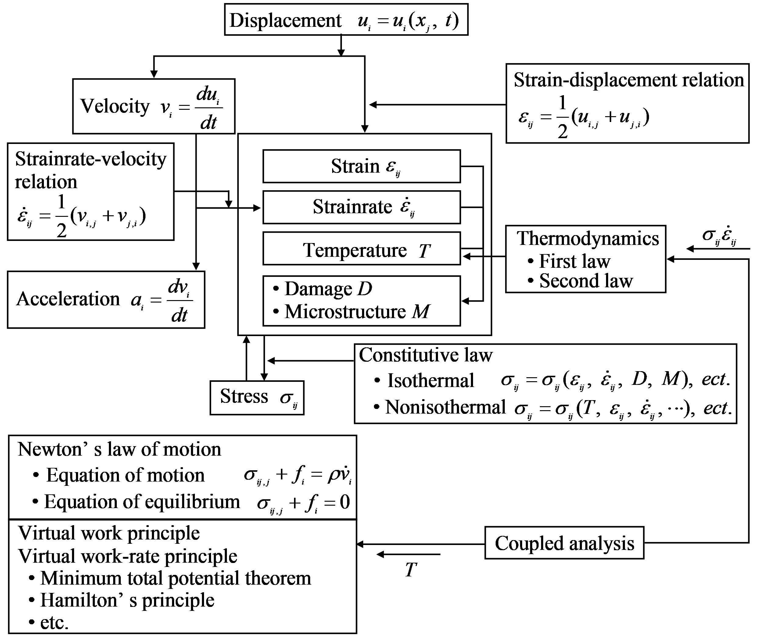
From the standpoint of the displacement method, solid mechanics is a discipline whose primary purpose is to determine displacement. The displacement of a solid consists largely of rigid-body motion and deformation. Rigid-body motion is divided into rigid-body translation and rigid-body rotation. Rigid-body motion is mainly treated in rigid-body dynamics. The dynamics learned in the lower years of university is, for the most part, rigid-body dynamics. In rigid-body motion, displacement is a function of time, and acceleration and kinetic energy have a great influence on the development of the theory. Deformation refers to what remains of displacement after rigid-body motion is excluded. Deformation induces relative displacement among particles and is expressed as a function of time and position.
Problems in which deformation is a function of time are mainly treated in dynamics in the broad sense (vibration, flexible-body dynamics), whereas problems in which deformation is static or quasi-static are treated in solid mechanics in the narrow sense (elasticity, plasticity, etc.). In the former, the effect of acceleration is reflected, whereas in the latter, the effect of acceleration is neglected. Materials behave differently according to their type and the conditions of use. Structural materials are used within the elastic range, whereas metal forming entails plastic deformation of a much larger magnitude than the elastic deformation. Solid mechanics in the elastic regime is called elasticity, and the field of study that deals with problems involving plastic deformation is called plasticity.
Mechanics problems are generally formulated as initial-boundary value problems. Plasticity is no exception. Boundary conditions are divided into essential boundary conditions and natural boundary conditions. In mechanics, essential boundary conditions correspond to geometric constraint conditions, whereas natural boundary conditions are boundary conditions related to loads. In heat transfer problems, the essential boundary condition is a boundary on which the temperature is prescribed, whereas the natural boundary condition is a boundary on which the heat transfer rate is prescribed. In general, every point on the boundary belongs to either an essential boundary condition or a natural boundary condition. When the unknown is a vector quantity such as a displacement field or a velocity field, as many boundary conditions as the number of dimensions of the vector quantity are imposed at a point on the boundary. For example, in a three-dimensional elasticity problem, boundary conditions must be imposed for all coordinate-axis directions at a point on the boundary, so three boundary conditions must be given independently.
The plasticity described above presupposes solving differential equations numerically. Before the introduction of numerical methods, approximate solution techniques based on analytical methods formed the mainstream of plasticity. Representative analytical approaches include the slab method, the slip-line method, and the upper-bound method [1.2-1.6]. These are still usefully employed for problems requiring closed-form solutions, such as rolling process control.