8 Finite Element Formulation of Deformation Problems

8.1 Introduction and Definition of the Boundary Value Problem

Figure 8.1 shows the flow chart and concept of a general metal-forming simulation. As shown in Figure 8.1, a metal-forming simulation consists of a preprocessor, a solver, and a post-processor.

Figure 8.1 Metal-forming simulation

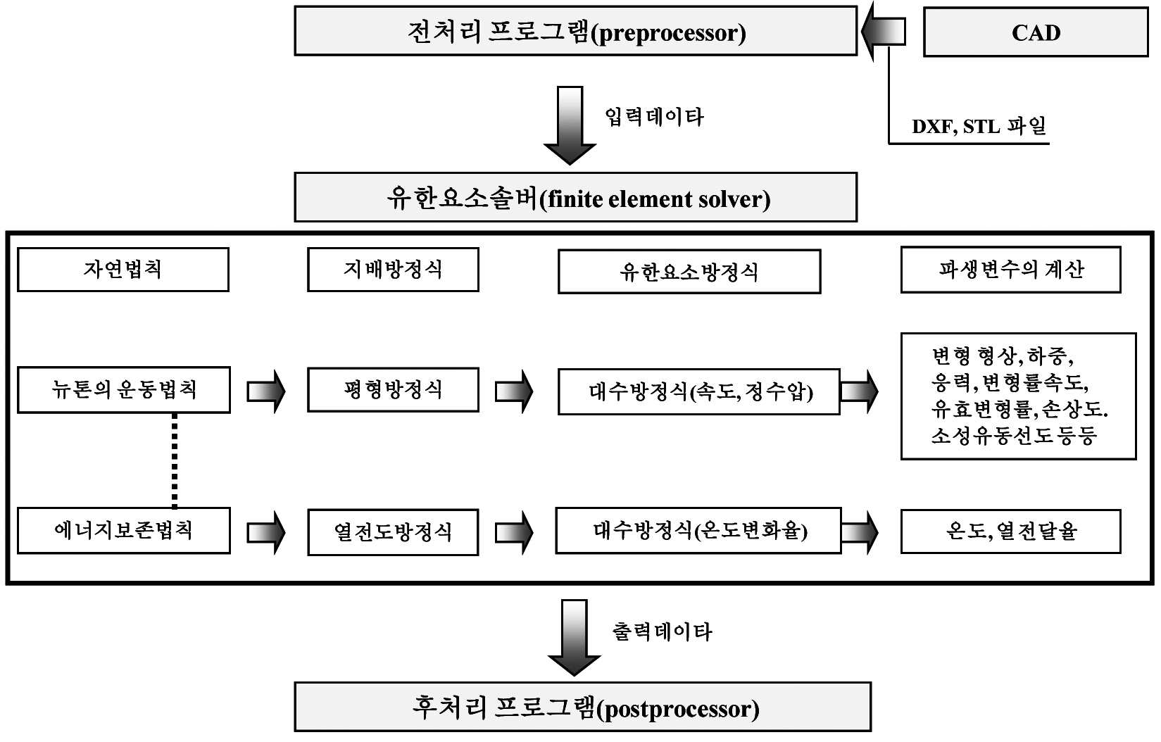
The preprocessor is basically connected to a CAD system and is supported by databases (DBs) of materials, presses, friction, and so on. The solver plays the role of obtaining unknowns such as velocity, pressure, and temperature so as to satisfy the process conditions required by the user. The post-processor helps the user readily turn the aforementioned unknowns—and the strain rate, deformation, stress, forming load, and other information derived from them—into usable information. The pre- and post-processors are evaluated by their ease of use, whereas the solver is evaluated by the accuracy of its results, computation speed, and versatility of application.

Information such as materials, presses, and friction basically belongs to the user's domain. Of course, the software provides basic information, but ultimately an attitude of continually expanding the DB to suit the user's environment is required. In particular, the flow stress of the material governs the results, and it is necessary to recognize that the material properties—that is, the macroscopic behavioral characteristics of the material—differ from country to country and from manufacturer to manufacturer, and that these properties change relatively significantly depending on pre-treatments such as heat treatment and drawing, as well as on the forging conditions.

A metal-forming simulation can be summarized as follows: the equilibrium equations and the heat conduction equation, which are derived as partial differential equations from natural laws, are discretized using finite element techniques to form nonlinear equations; by solving these, the velocity, pressure (in the Lagrange multiplier method), rate of temperature change, and so on are obtained first, and from these various derived variables such as strain rate, deformed shape, and temperature distribution are obtained.

Analysis information is broadly divided into process-geometry information, process-condition information, and material-property information. Process-geometry information includes the process layout, die shape, workpiece shape, and so on. Process-condition information, or process conditions, includes data such as friction, die velocity, and heat transfer coefficient. And material-property information includes the flow stress, thermal conductivity, heat capacity, and so on of the material. In addition, items that the analysis engineer must determine or define include symmetry-plane information, stroke information, the number of elements, the equation solution method, and so on. This chapter summarizes the contents of reference [1.1] and adds new material as needed.

8.2 Rigid-Plastic Finite Element Method

8.2.1 Definition of the Rigid-Plastic Deformation Problem

The metal-forming material is assumed to have properties such as incompressibility, rigid-plasticity, and isotropic hardening, to follow the Huber-von Mises yield theory and the associated flow rule, and to follow the Coulomb friction law, the constant shear friction law, the hybrid friction law, and so on at the contact surface. Furthermore, the effects of self-weight and acceleration are assumed to be negligibly small.

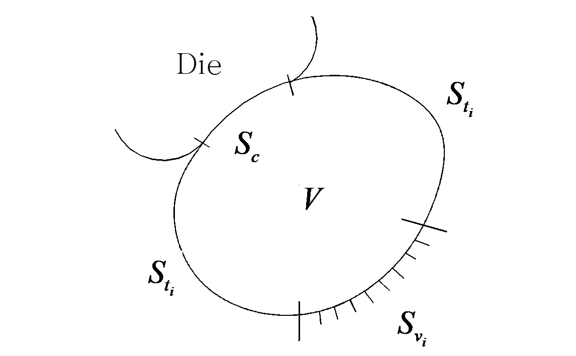
As shown in Figure 8.2, in a metal-forming process the die and the workpiece are divided into the analysis domain \(V\) and the boundary \(S\), and the boundary \(S\) can be subdivided into \(S_{t_i}\) where the traction is prescribed as \(t_i^{(n)} = \bar{t}_i^{(n)}\), \(S_{v_i}\) where the velocity is prescribed as \(v_i = \bar{v}_i\), \(S_c\) representing the contact surface between the die and the workpiece, and so on. At the contact between the die and the workpiece where compressive force acts, the normal velocities are equal. That is, on \(S_c\), \(v_n = \bar{v}_n\).

The flow analysis problem of a metal-forming process seeks the velocity field \(v_i\) and the hydrostatic pressure \(p\) (in the Lagrange multiplier method), or the velocity field \(v_i\) (in the penalty method) of the workpiece, and is formulated as the following boundary value problem.

Figure 8.2 Conceptual diagram of the plasticity-mechanics problem

(1) Equilibrium equation

\[ \sigma_{ij,j} + f_i = 0 \tag{8.1} \]

(2) Stress–strain-rate relation

\[ \sigma_{ij} = -p \delta_{ij} + \sigma'_{ij} \tag{8.2} \]

\[ \sigma'_{ij} = \frac{2\bar{\sigma}}{3\dot{\bar{\varepsilon}}} \dot{\varepsilon}_{ij} \tag{8.3} \]

(3) Velocity–strain-rate relation

\[\dot{\varepsilon}_{ij} = \frac{1}{2}(v_{i,j} + v_{j,i}) \tag{8.4}\]

(4) Incompressibility condition

\[v_{i,i} = 0 \tag{8.5}\]

(5) Boundary conditions

\[\sigma_{ij}n_j = \bar{t}_i^{(n)} \quad \text{on} \quad S_{t_i} \tag{8.6}\]

\[v_i = \bar{v}_i \quad \text{on} \quad S_{v_i} \tag{8.7}\]

\[v_n = \bar{v}_n \quad \text{on} \quad S_c \tag{8.8}\]

\[\sigma_t = -\mu\sigma_n g(v_t) \quad \text{on} \quad S_c \quad \text{(Coulomb friction)} \tag{8.9}\]

\[\sigma_t = mkg(v_t) \quad \text{on} \quad S_c \quad \text{(constant shear friction)} \tag{8.10}\]

\[\sigma = \min(-\mu\sigma_n, m'k)g(v_t) \quad \text{on} \quad S_c \quad \text{(hybrid friction)} \tag{8.11}\]

Here \(\min(*, *)\) means taking the smaller of the two values, and \(m'\) is a constant for constraining the maximum value of the friction stress, that is, the limiting friction constant. In the equilibrium equation, \(f_i\) is the body force. In the constitutive equation, \(\bar{\sigma}\) and \(\dot{\bar{\varepsilon}}\) denote the flow stress and the effective strain rate, respectively. In general, the flow stress in Equation (8.3),

\[ \bar{\sigma} = \bar{\sigma}(\bar{\varepsilon}, \dot{\bar{\varepsilon}}, T) \tag{8.12} \]

is a function of the strain \(\bar{\varepsilon}\), the strain rate \(\dot{\bar{\varepsilon}}\), the temperature \(T\), and so on, and is a function that reflects the mechanical properties or state of the material. The vector \(n_i\) in Equation (8.6) is defined on the analysis boundary and is the outward unit normal vector. In tensor quantities, the superscript prime (\('\)) denotes the deviatoric component, and the subscripts \(t\) and \(n\) denote the tangential and normal components, respectively. A repeated subscript follows the summation convention, and a subscript following a comma (,) denotes partial differentiation. These conventions apply to all equations. In Equations (8.9) and (8.10), \(g(v_t)\) is given by the following.

\[g(v_t) = -\frac{2}{\pi} \tan^{-1} \left( \frac{v_t - \bar{v}_t}{a} \right) \tag{8.13}\]

Here \(a\) is a very small positive constant compared with \(|v_t|\).

When the penalty method is used and when the Lagrange multiplier method is used to treat the incompressibility condition, the weak forms of the above boundary value problem are, respectively, as follows [1.1].

\[\int_V \sigma'_{ij} \omega'_{ij} dV + \int_V K \dot{\varepsilon}_{ii} \omega_{jj} dV - \int_V f_i \omega_i dV - \sum \int_{S_{t_i}} \bar{t}_i^{(n)} \omega_i dS - \int_{S_c} \sigma_t \omega_t dS = 0 \tag{8.14}\]

\[\int_V \sigma'_{ij} \omega'_{ij} dV - \int_V p \omega_{jj} dV - \int_V f_i \omega_i dV - \int_V v_{i,i} q dV - \sum \int_{S_{t_i}} \bar{t}_i^{(n)} \omega_i dS - \int_{S_c} \sigma_t \omega_t dS = 0 \tag{8.15}\]

Here the weighting function \(\omega_i\) is an arbitrary function that takes the value zero on the boundary \(S_{v_i}\), and the weighting function \(q\) is an arbitrary function over the entire analysis domain. In the weak form,

\[\omega_{ij} = \left( \frac{\omega_{i,j} + \omega_{j,i}}{2} \right) \tag{8.16}\]

and \(\omega_n\) and \(\omega_t\) denote the normal and tangential components of \(\omega_i\), respectively. In the penalty method, the penalty constant \(K\) has the following physical meaning.

\[K \dot{\varepsilon}_{ii} = \sigma_{jj} / 3 = -p \tag{8.17}\]

Therefore, in the penalty method the pressure distribution is obtained from the velocity-field analysis result. In conclusion, solving the aforementioned boundary value problem is, when the Lagrange multiplier method is used, the problem of finding the velocity field \(v_i\) and the pressure \(p\) that always satisfy the weak form, that is, Equation (8.15), for arbitrary weighting functions \(\omega_i\) and \(q\); and when the penalty method is used, it is formulated as the problem of finding the velocity field \(v_i\) that always satisfies the weak form, that is, Equation (8.14), for an arbitrary weighting function \(\omega_i\). Of course, the velocity field must satisfy the essential boundary conditions on \(S_{v_i}\) and \(S_c\).

In the Lagrange multiplier method, the velocity field \(v_i\) and the pressure \(p\), and the weighting functions \(\omega_i\) and \(q\), form the basis of the weak form. Everything else is derived from them. Therefore, by interpolating these four functions, a nonlinear system of equations in which the nodal velocities and the elemental pressures are the unknowns can be obtained. In the penalty method, by interpolating the velocity field \(v_i\) and the weighting function \(\omega_i\), a nonlinear system of equations in which the nodal velocities are the unknowns can be obtained. Basic knowledge of the finite element method is provided in Appendix B. In this book, the derivation of the finite element equations of the rigid-plastic finite element method is left to reference [1.1], whereas that process for the elasto-plastic finite element method is detailed in Section 8.3.

8.2.2 Minimum Effective Strain Rate

The denominator of Equation (8.3) contains the effective strain rate \(\dot{\bar{\varepsilon}}\). This value is theoretically 0.0 in the elastic region, at which point numerical computation becomes impossible. To resolve this problem, when the effective strain rate falls below an allowable minimum effective strain rate, this allowable minimum effective strain rate is used instead of that value. This value can have a large effect on the accuracy and convergence characteristics of the analysis results. If this value is set large, the solution will be obtained relatively easily, but it causes excessive numerical deformation in the characteristic region and therefore mostly plays a negative role of degrading the solution accuracy. Conversely, if this value is set very small, the solution is more likely to approach the theoretical solution, but the convergence characteristics of the solution deteriorate. Therefore, relatively careful attention is required in determining this value as well.

8.2.3 Die-Penetration Tolerance and Updating

In general, during a metal-forming simulation, when determining nodal positions based on velocity-field information, penetration of nodes into the die is allowed. If nodes are not allowed to penetrate the die, there is a problem that the advance of the analysis is slowed. Of course, the position of a penetrating node is either artificially corrected to a nearby point on the die surface, or, while maintaining the penetrated state, it is pushed out to the die surface. The former is not advantageous in terms of artificial volume change.

The allowable penetration depth of a node into the die has a non-negligible effect on the accuracy of the predicted results, the computation time, and so on. Experience suggests that it is desirable to set the allowable die-penetration depth of a node to 50% or less of the desired prediction accuracy. For example, when one wishes to analyze with an accuracy of 0.02 mm, it is desirable to allow 0.01 mm or less. If the penetrating-node push-out technique is used, this value may be increased up to threefold. Most programs set a default value to prevent large user mistakes. Since it is generally uncommon to require an accuracy of 0.001 mm from a metal-forming simulator, without careful attention this can become a problem when analyzing processes whose dimensions themselves are very small, such as micro-forming processes (see Appendix D.2.1). The more intelligent the program, the more severe this problem becomes.

8.3 Elasto-Plastic Finite Element Method

Rigid-plastic finite element analysis presumes that only plastic deformation occurs in a metallic material during metal forming. That is, elastic deformation is neglected. For observing the overall material flow, loads, and so on, rigid-plastic finite element analysis is often sufficient, and it is usefully employed in many cases owing to its advantages of short computation time and good convergence. During a metal-forming process the material undergoes elastic deformation simultaneously with plastic deformation, whereas rigid-plastic finite element analysis does not consider elastic deformation; therefore some degree of error is unavoidable in the calculation of stress and deformation, and the elastic recovery upon load removal cannot be calculated. Compared with rigid-plastic finite element analysis, elasto-plastic finite element analysis can resolve these problems, but it has the disadvantages of requiring more analysis time and being less favorable in terms of stably obtaining a solution. Therefore, it is desirable to use rigid-plastic finite element analysis and elasto-plastic finite element analysis appropriately according to the situation.

8.3.1 Definition of the Elasto-Plastic Deformation Problem

Figure 8.3 is a conceptual diagram of a metal-forming process for developing the finite element method for an elasto-plastic material, that is, the elasto-plastic finite element method. In a metal-forming process, the die and the workpiece can be divided into the analysis domain \(V\) and the boundary \(S\), and the boundary \(S\) can be represented as \(S_t\) where the traction is \(t_i^{(n)} = \bar{t}_i\), \(S_u\) where the displacement is prescribed as \(u_i = \bar{u}_i\), \(S_c\) representing the contact surface between the die and the workpiece, and so on. In the following theoretical development, the workpiece is restricted to the case in which it has properties such as isotropic elasto-plasticity, rate independence, and isotropic hardening, and follows the von Mises yield theory and the associated flow rule. In addition, assuming that a quasi-static phenomenon in which the effect of acceleration is negligible occurs during the process, the static implicit finite element method is described.

Figure 8.3 Definition of the elasto-plastic flow analysis problem

The metal-forming process problem for an elasto-plastic material seeks the displacement \(u_i\) of the workpiece, and is formulated as the following boundary value problem.

(1) Equilibrium equation

\[\sigma_{ij,j} + f_i = 0 \quad \text{in} \quad V \tag{8.18}\]

(2) Decomposition of the strain increment

\[d\varepsilon_{ij} = d\varepsilon_{ij}^e + d\varepsilon_{ij}^p \tag{8.19}\]

(3) Constitutive equations

\[\text{Elastic} : d\varepsilon_{ij}^e = \frac{d\sigma'_{ij}}{2G} + \frac{1-2\nu}{E} d\sigma_m \delta_{ij} \tag{8.20}\]

\[\text{Plastic} : d\varepsilon_{ij}^p = d\lambda \frac{\partial f}{\partial \sigma_{ij}} = \frac{3}{2} d\lambda \frac{\sigma'_{ij}}{\bar{\sigma}} \tag{8.21}\]

(4) Displacement–strain-increment relation

\[d\varepsilon_{ij} = \frac{1}{2} \left( \frac{\partial u_i}{\partial x_j} + \frac{\partial u_j}{\partial x_i} \right) \tag{8.22}\]

(5) Yield function

\[f = \sigma_e - \sigma_y = \left( \frac{3}{2} \sigma'_{ij} \sigma'_{ij} \right)^{\frac{1}{2}} - \sigma_y = 0 \tag{8.23}\]

(6) Incompressibility condition

\[d\varepsilon_{ii}^p = 0 \tag{8.24}\]

(7) Boundary conditions

\[\sigma_{ij}n_j = \bar{t}_i \quad \text{on} \quad S_t \tag{8.25}\]

\[u_i = \bar{u}_i \quad \text{on} \quad S_u \tag{8.26}\]

\[u_n = \bar{u}_n \quad \text{on} \quad S_c \tag{8.27}\]

\[\sigma_t = -\mu\sigma_n g(v_t) \quad \text{on} \quad S_c \tag{8.28}\]

Here the superscripts \(p\) and \(e\) are indices denoting the plastic component and the elastic component, respectively. Also, the subscripts \(n\) and \(t\) are indices denoting the normal component and the tangential component, respectively. The strain increment \(d\varepsilon_{ij}\) is obtained taking the rotation of the material into account, and the description is restricted to the case in which the size of one computation increment is small enough to be computed after linearization. The \(g(v_t)\) in Equation (8.28) is a function reflecting the relationship between friction and velocity, and is explained in the previous section. Furthermore, the application of Equation (8.22) is limited to the case of a small strain increment, and the method of considering large deformation involving a large strain increment and large rotation is described in 8.3.7.

8.3.2 von Mises Yield Function

The \(d\lambda\) in Equation (8.21) can be obtained simply in the case of the von Mises yield function. In Equation (8.21),

\[d\varepsilon_{ij}^p = \frac{3}{2} d\lambda \frac{\sigma'_{ij}}{\bar{\sigma}} \tag{8.29}\]

and the effective plastic strain increment \(d\bar{\varepsilon}^p\) is given by the following equation.

\[d\bar{\varepsilon}^p = \left( \frac{2}{3} d\varepsilon_{ij}^p d\varepsilon_{ij}^p \right)^{\frac{1}{2}} \tag{8.30}\]

Substituting Equation (8.29) into Equation (8.30),

\[d\bar{\varepsilon}^p = \left( \frac{2}{3} \frac{3}{2} d\lambda \frac{\sigma'_{ij}}{\bar{\sigma}} \frac{3}{2} d\lambda \frac{\sigma'_{ij}}{\bar{\sigma}} \right)^{\frac{1}{2}} = d\lambda \frac{\left( \frac{3}{2} \sigma'_{ij} \sigma'_{ij} \right)^{\frac{1}{2}}}{\bar{\sigma}} = d\lambda \tag{8.31}\]

That is, in the case of the von Mises yield function, \(d\lambda\) is found to be identical to the effective plastic strain increment \(d\bar{\varepsilon}^p\). Therefore, the plastic flow rule of Equation (8.21) can be rewritten as follows.

\[d\varepsilon_{ij}^p = \frac{3}{2} d\bar{\varepsilon}^p \frac{\sigma'_{ij}}{\bar{\sigma}} \tag{8.32}\]

8.3.3 Isotropic Work Hardening and the Consistency Condition

Most metals harden as they undergo the plastic deformation process. That is, a larger stress is required to induce further plastic deformation. The effective plastic strain \(\bar{\varepsilon}^p\) is integrated along the deformation path as in the following equation.

\[\bar{\varepsilon}^p = \int d\bar{\varepsilon}^p \tag{8.33}\]

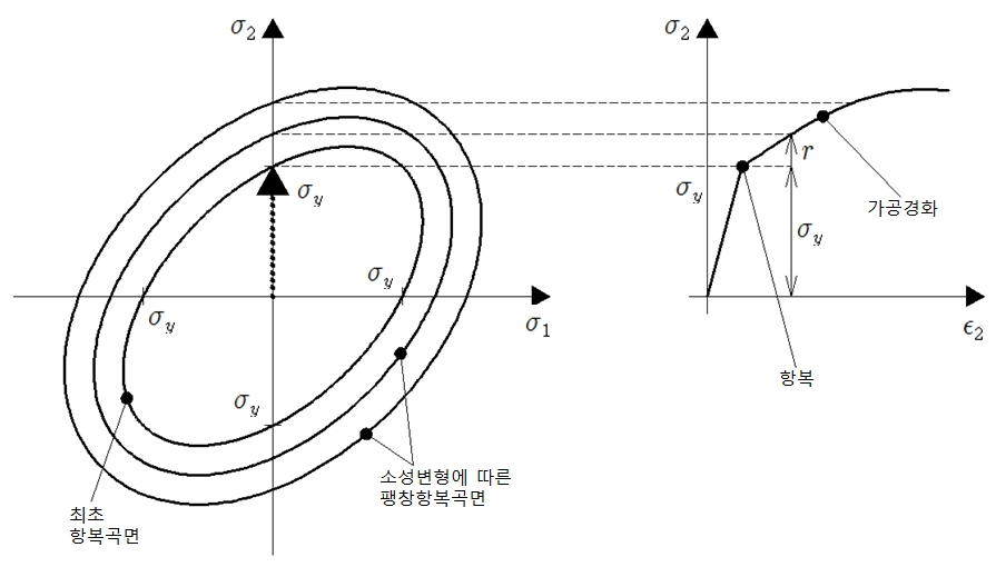
Here \(d\bar{\varepsilon}^p\) is given by Equation (8.30). Figure 8.4 shows the strain–stress curve in uniaxial tension in which work hardening occurs under a plane-stress condition, and the resulting initial yield surface and the yield surface that progressively expands with work hardening. At this time, if yielding occurs at the same magnitude of stress in all other directions, including directions of different sign, then isotropy holds and the material is said to have the characteristic of isotropic work hardening. In Figure 8.4, as the stress initially increases in the two-axis direction, only elastic deformation occurs until the initial yield surface is reached. As the stress gradually increases and \(\sigma_2 = \sigma_y\), yielding occurs. As the deformation proceeds further, the workpiece work-hardens, and since the amount of work hardening can be expressed by the effective plastic strain \(\bar{\varepsilon}^p\), the yield function of Equation (8.23) can be expressed as the following equation.

\[f(\sigma, \bar{\varepsilon}^p) = \sigma_e - \sigma_y(\bar{\varepsilon}^p) = 0 \tag{8.34}\]

Figure 8.4 Isotropic work hardening

Here \({\sigma}\) is the stress tensor. Meanwhile, in uniaxial tension the above equation becomes identical to the following equation.

\[\sigma_e - \sigma_y(\bar{\varepsilon}^p) = \sigma_2 - \sigma_y(\varepsilon_2^p) = 0 \tag{8.35}\]

Therefore, in Figure 8.4, as \(\varepsilon_2^p (=\bar{\varepsilon}^p)\) increases, the flow stress \(\sigma_2 (=\sigma_e)\) must be increased so that the yield surface, whose size is determined by the effective stress, also increases to satisfy the yield function, in order for yielding to continue. In Figure 8.4, \(r\) denotes the amount of work hardening. In this way, when work hardening occurs, for plastic deformation to continue, the stress must lie on the yield surface, and this is called the consistency condition.

8.3.4 Formulation of the Elasto-Plastic Finite Element Method

For an arbitrary variation of displacement \(\delta{\omega}\) that becomes zero on the boundary where the displacement field is prescribed, the weak form for finding the displacement field \(\mathbf{u}\) is as follows.

\[\int_V \delta\varepsilon_{ij}\sigma_{ij} dV - \int_V \delta\omega_i f_i dV - \int_{S_t} \delta\omega_i t_i dS - \int_{S_c} \delta\omega_t \sigma_t dS = 0 \tag{8.36}\]

Here \(f_i\) and \(t_i\) denote the body-force component and the traction component, respectively.

The displacement and the weighting function (or virtual displacement) within a finite element are approximated using interpolation functions (or shape functions) as follows.

\[\mathbf{u} = \mathbf{N}\mathbf{U} \tag{8.37}\]

\[{\omega} = \mathbf{N}\mathbf{W} \tag{8.38}\]

Here \(\mathbf{N}\) is a matrix containing the interpolation functions that approximate the displacement within the element. \(\mathbf{U}\) and \(\mathbf{W}\) are vectors representing the nodal values of the displacement and the weighting function.

The stress tensor \({\sigma} = [\sigma_{ij}]\) and the strain tensor \({\varepsilon} = [\varepsilon_{ij}]\) are expressed in vector form as in the following equation and used in the finite element formulation.

\[\tilde{{\sigma}} = \begin{bmatrix} \sigma_{xx} \\ \sigma_{yy} \\ \sigma_{zz} \\ \sigma_{xy} \\ \sigma_{yz} \\ \sigma_{zx} \end{bmatrix}, \quad \tilde{{\varepsilon}} = \begin{bmatrix} \varepsilon_{xx} \\ \varepsilon_{yy} \\ \varepsilon_{zz} \\ \varepsilon_{xy} \\ \varepsilon_{yz} \\ \varepsilon_{zx} \end{bmatrix} \tag{8.39}\]

The strain increment can be expressed by the following equation using Equations (8.39) and (8.37).

\[d\tilde{{\varepsilon}} = \begin{bmatrix} d\varepsilon_{xx} \\ d\varepsilon_{yy} \\ d\varepsilon_{zz} \\ 2d\varepsilon_{xy} \\ 2d\varepsilon_{yz} \\ 2d\varepsilon_{zx} \end{bmatrix} = \frac{\partial \mathbf{N}}{\partial \mathbf{x}} \mathbf{U} = \mathbf{B}\mathbf{U} \tag{8.40}\]

In elasto-plastic analysis, the stress increment \(\Delta{\sigma}\) is given in the following form.

\[d\tilde{{\sigma}} = \tilde{\mathbf{C}}^{ep} d\tilde{{\varepsilon}} \tag{8.41}\]

Here \(\tilde{\mathbf{C}}^{ep}\) is used by reducing the order of the fourth-order tensor \(\mathbf{C}^{ep}\) in Equation (8.61) to second order. Equation (8.36) is rearranged as follows.

\[\int_V \delta\tilde{{\varepsilon}}^T \tilde{{\sigma}} dV - \int_V \delta{\omega}^T \mathbf{f} dV - \int_{S_t} \delta{\omega}^T \mathbf{t}^{(n)} dS - \int_{S_c} \delta\omega_t \tilde{\sigma}_t dS = 0 \tag{8.42}\]

In elasto-plastic analysis, in order to account for nonlinearity, the computation must be divided into several computation increments and performed sequentially. When the solution has been obtained at time \(t_n\), in order to obtain the solution at time \(t_{n+1}\), the following equation can be obtained by applying Equation (8.41) to Equation (8.42) for the deformation over the time-increment interval \(\Delta t = t_{n+1} - t_n\).

\[\int_V \delta \tilde{\varepsilon}^T (\tilde{\sigma}_n + \tilde{\mathbf{C}}^{ep} d\tilde{\varepsilon}) dV - \int_V \delta \omega^T \mathbf{f} dV - \int_{S_t} \delta \omega^T \mathbf{t}^{(n)} dS - \int_{S_c} \delta \omega_t \tilde{\sigma}_t dS = 0 \tag{8.43}\]

Applying Equations (8.37), (8.38), and (8.40) to Equation (8.43) gives the following.

\[\int_V \delta(\mathbf{B}\mathbf{W})^T (\tilde{\sigma}_n + \tilde{\mathbf{C}}^{ep}\mathbf{B}\mathbf{U}) dV - \int_V \delta(\mathbf{N}\mathbf{W})^T \mathbf{f} dV - \int_{S_t} \delta(\mathbf{N}\mathbf{W})^T \mathbf{t}^{(n)} dS - \int_{S_c} \delta(\mathbf{N}\mathbf{W})^T \mathbf{t} \tilde{\sigma}_t dS = 0 \tag{8.44}\]

\[\delta \mathbf{W}^T \left[ \int_V \mathbf{B}^T (\tilde{\sigma}_n + \tilde{\mathbf{C}}^{ep} \mathbf{B}\mathbf{U}) dV - \int_V \mathbf{N}^T \mathbf{f} dV - \int_{S_t} \mathbf{N}^T \mathbf{t}^{(n)} dS - \int_{S_c} \mathbf{N}^T \mathbf{t} \tilde{\sigma}_t dS \right] = 0 \tag{8.45}\]

Since it must hold for arbitrary \(\delta \mathbf{W}\), the following equation is obtained.

\[\int_V \mathbf{B}^T (\tilde{\sigma}_n + \tilde{\mathbf{C}}^{ep} \mathbf{B}\mathbf{U}) dV - \int_V \mathbf{N}^T \mathbf{f} dV - \int_{S_t} \mathbf{N}^T \mathbf{t}^{(n)} dS - \int_{S_c} \mathbf{N}^T \mathbf{t} \tilde{\sigma}_t dS = 0 \tag{8.46}\]

Rearranging Equation (8.46) gives the following finite element equation.

\[[\mathbf{K}]\{\mathbf{U}\} + \{\mathbf{F}^n\} - \{\mathbf{F}^{ext}\} = 0 \tag{8.47}\]

Here

\[[\mathbf{K}] = \int_V \mathbf{B}^T \tilde{\mathbf{C}}^{ep} \mathbf{B} dV \tag{8.48}\]

\[\mathbf{F}^{ext} = \int_V \mathbf{N}^T \mathbf{f} dV + \int_{S_t} \mathbf{N}^T \tilde{\mathbf{t}} dS + \int_{S_c} \mathbf{N}^T \mathbf{t} \tilde{\sigma}_t dS \tag{8.49}\]

\[\mathbf{F}^n = \int_V \mathbf{B}^T \tilde{\sigma}_n dV \tag{8.50}\]

Owing to the various nonlinearities in a metal-forming process, the solution satisfying Equation (8.47) is obtained by applying the Newton-Raphson iteration method. The residual force arising in Equation (8.47) is expressed by the following equation.

\[\Psi(\mathbf{U}) = [\mathbf{K}]\{\mathbf{U}\} + \{\mathbf{F}^n\} - \{\mathbf{F}^{ext}\} \tag{8.51}\]

Approximating Equation (8.51) by the Taylor method gives the following equation.

\[\Psi(\mathbf{U}) + \frac{\partial \Psi(\mathbf{U})}{\partial \mathbf{U}} \Delta\mathbf{U} + O(\Delta\mathbf{U}^2) = 0 \tag{8.52}\]

Here the matrix \(\mathbf{J} = \partial \Psi / \partial \mathbf{U}\) is called the Jacobian, or the effective tangent stiffness matrix. Linearizing by using only the first-order term in Equation (8.52) gives the following equation.

\[\frac{\partial \Psi(\mathbf{U})}{\partial \mathbf{U}} \Delta\mathbf{U} = \mathbf{J}(\mathbf{U}) \Delta\mathbf{U} = -\Psi(\mathbf{U}) \tag{8.53}\]

The iterative computation in Equation (8.53) continues until the residual force of Equation (8.51) decreases below a predetermined threshold. During the iterative computation, the displacement \(\mathbf{U}\) is updated as follows. Here \(m\) denotes the iteration count.

\[\mathbf{J}(\mathbf{U}_m) \Delta\mathbf{U}_m = -\Psi(\mathbf{U}_m) \tag{8.54}\]

\[\mathbf{U}_{m+1} = \mathbf{U}_m + \Delta\mathbf{U}_m \tag{8.55}\]

8.3.5 Integration of Stress and State Variables

When obtaining a numerical solution, as the plastic deformation progresses, the stress, strain, state variables, and so on must be integrated with respect to the deformation time so as to satisfy the relevant equations. The integration can be performed by an explicit integration method or an implicit integration method.

When a stress increment and the resulting effective plastic strain increment occur, the condition for maintaining consistency can be stated as follows.

\[f(\sigma + d\sigma, \bar{\varepsilon}^p + d\bar{\varepsilon}^p) = 0 \tag{8.56}\]

Expanding Equation (8.56),

\[f(\sigma + d\sigma, \bar{\varepsilon}^p + d\bar{\varepsilon}^p) = f(\sigma, \bar{\varepsilon}^p) + \frac{\partial f}{\partial \sigma} : d\sigma + \frac{\partial f}{\partial \bar{\varepsilon}^p} d\bar{\varepsilon}^p = 0 \tag{8.57}\]

Here the operator ( : ) performs a tensor contraction to compute a scalar value. For Equation (8.57) to hold, the following equation must be satisfied.

\[\mathbf{n} : d\sigma + \frac{\partial f}{\partial \bar{\varepsilon}^p} d\bar{\varepsilon}^p = 0 \tag{8.58}\]

Here

\[\mathbf{n} = \frac{\partial f}{\partial \sigma} \tag{8.59}\]

Using Hooke's law, the relation between the stress increment and the elastic strain increment can be obtained.

\[d\sigma = \mathbf{C} d\varepsilon^e = \mathbf{C}(d\varepsilon - d\varepsilon^p) \tag{8.60}\]

Here \(\mathbf{C}\) is a fourth-order tensor representing the elastic deformation relation between the stress tensor and the strain tensor. Using the expression for the plastic strain increment \(d\varepsilon^p\) in Equation (8.21), the following can be obtained.

\[d\sigma = \mathbf{C} d\varepsilon^e = \mathbf{C}(d\varepsilon - d\lambda \mathbf{n}) \tag{8.61}\]

And applying Equations (8.31) and (8.61) to Equation (8.58) gives the following equation.

\[\mathbf{n} : \{\mathbf{C}(d\varepsilon - d\lambda \mathbf{n})\} + \frac{\partial f}{\partial \bar{\varepsilon}^p} d\lambda = 0 \tag{8.62}\]

From this equation, an equation for \(d\lambda\) can be obtained as follows.

\[d\lambda = \frac{\mathbf{n} : \mathbf{C} d\varepsilon}{\mathbf{n} : \mathbf{C}\mathbf{n} - \left( \frac{\partial f}{\partial \bar{\varepsilon}^p} \right)} \tag{8.63}\]

Substituting Equation (8.63) into Equation (8.61) and rearranging gives the following equation for the stress increment.

\[d\sigma = \mathbf{C} \left( d\varepsilon - \mathbf{n} \frac{\mathbf{n} : \mathbf{C} d\varepsilon}{\mathbf{n} : \mathbf{C}\mathbf{n} - \left( \frac{\partial f}{\partial \bar{\varepsilon}^p} \right)} \right) = \left( \mathbf{C} - \frac{(\mathbf{C} : \mathbf{n}) \otimes (\mathbf{C} : \mathbf{n})}{\mathbf{n} : \mathbf{C}\mathbf{n} - \left( \frac{\partial f}{\partial \bar{\varepsilon}^p} \right)} \right) d\varepsilon \tag{8.64}\]

or

\[d\sigma = \mathbf{C}^{ep} d\varepsilon \tag{8.65}\]

Here \(\mathbf{C}^{ep}\) denotes the elasto-plastic tangent stiffness. The operator ( \(\otimes\) ) denotes the tensor product (or dyadic). When there is no plastic deformation, \(d\lambda = 0\), and in that case \(\mathbf{C}^{ep} = \mathbf{C}\), reverting to the case of elastic deformation.

In Equation (8.65), the method of computing the physical quantities at the next time step \(t_{n+1}\) using only the values at time \(t_n\)—when the total deformation increment \(d\varepsilon\) is given and the stress \(\sigma_{t_n}\) and the work-hardening state variable \(\bar{\varepsilon}_{t_n}^p\) at the previous time step \(t_n\) are given—is called the explicit integration method. Using the above equations, the necessary values are computed using the values at the step time \(t_n\).

\[d\lambda_{t_n} = \frac{\mathbf{n}_{t_n} : \mathbf{C} d\varepsilon_{t_n}}{\mathbf{n}_{t_n} : \mathbf{C}\mathbf{n}_{t_n} - \left( \frac{\partial f}{\partial \bar{\varepsilon}^p} \right)_{t_n}} \tag{8.66}\]

\[d\sigma_{t_n} = \mathbf{C} \left( d\varepsilon_{t_n} - d\lambda_{t_n} \mathbf{n}_{t_n} \right) \tag{8.67}\]

\[dr_{t_n} = \frac{\partial f}{\partial \bar{\varepsilon}_{t_n}^p} d\bar{\varepsilon}_{t_n}^p \tag{8.68}\]

By time integration, the values at time \(t_{n+1}\) are obtained as follows.

\[\sigma_{t_{n+1}} = \sigma_{t_n} + d\sigma_{t_n} \tag{8.69}\]

\[\varepsilon_{t_{n+1}}^p = \varepsilon_{t_n}^p + d\varepsilon_{t_n}^p \tag{8.70}\]

\[r_{t_{n+1}} = r_{t_n} + dr_{t_n} \tag{8.71}\]

This integration method is the first-order forward-Euler explicit integration method, and while it can be implemented simply, it has various disadvantages. The time increment must be sufficiently small for the solution not to become unstable, and the accuracy is also greatly affected by the size of the time increment. In addition, there is no guarantee that the final stress state satisfies the consistency condition of lying on the yield surface.

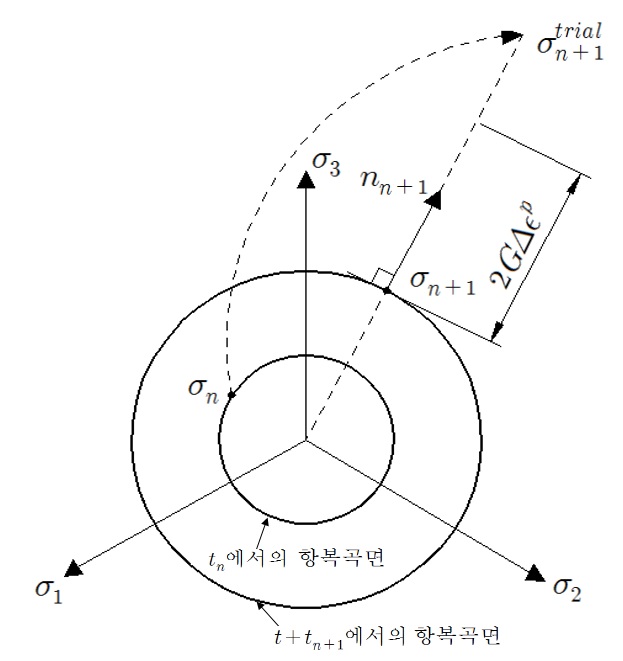
Therefore, in order to satisfy the consistency condition at time \(t_{n+1}\), an implicit integration method must be used. Figure 8.5 shows the process of making the stress state lie on the von Mises yield surface at time \(t_{n+1}\) using the implicit integration method. In three-dimensional stress space, the von Mises yield surface appears as a cylindrical surface whose central axis coincides with the line representing the hydrostatic stress. Figure 8.5 depicts the stress space projected in the direction parallel to that line, and in this case the von Mises yield surface appears as a circle. In the implicit integration process, the stress \(\mathbf{\sigma}_{n+1}^{tr} (= \mathbf{\sigma}_{n+1}^{trial})\) is first predicted elastically. \(\mathbf{\sigma}_{n+1}^{tr}\) generally does not coincide with the yield surface at the time whose size has changed due to work hardening. In this case, for the von Mises yield surface, it can be simply made to coincide with the new yield surface by returning it toward the center of the yield surface, which appears as a circle as in Figure 8.5. The stress correction component in this case is the plastic correction component, corresponding to \(2G\Delta\varepsilon^p\) in Figure 8.5. This method is called the radial return method [8.1], and in the case of the von Mises yield surface it can be performed very simply. The radial return method is explained below, and for readability, the time subscript is omitted for the terms corresponding to time \(t_{n+1}\) in the following equations.

Figure 8.5 Implicit stress integration process of the von Mises yield function from t_n to t_n+1

Using Hooke's law, an equation for the elastic stress can be obtained as follows.

\[\sigma = 2G\varepsilon^e + \lambda Tr(\varepsilon^e)\mathbf{I} \tag{8.72}\]

Here \(\mathbf{I}\) denotes the identity matrix. At time \(t_{n+1}\), the elastic strain can be written as follows.

\[\varepsilon^e = \varepsilon_{t_n}^e + \Delta\varepsilon^e = \varepsilon_{t_n}^e + \Delta\varepsilon - \Delta\varepsilon^p \tag{8.73}\]

Substituting Equation (8.73) into Equation (8.72),

\[\sigma = 2G(\varepsilon_{t_n}^e + \Delta\varepsilon) + \lambda Tr(\varepsilon_{t_n}^e + \Delta\varepsilon)\mathbf{I} - 2G\Delta\varepsilon^p = \sigma^{tr} - 2G\Delta\bar{\varepsilon}^p \mathbf{n} \tag{8.74}\]

Equation (8.74) can be divided into the hydrostatic stress component and the deviatoric stress component \(\sigma'\) and written as follows.

\[\sigma' + \frac{1}{3}(\sigma:\mathbf{I}) = \sigma'^{tr} - 2G\Delta\bar{\varepsilon}^p \frac{3}{2}\frac{\sigma'}{\sigma_e} \tag{8.75}\]

Rearranging Equation (8.75),

\[\left( 1 + 3G\frac{\Delta\bar{\varepsilon}^p}{\sigma_e} \right)\sigma' = \sigma'^{tr} \tag{8.76}\]

Squaring both sides of the above equation and rearranging using Equation (8.23) gives the following equation.

\[\sigma_e + 3G\Delta\bar{\varepsilon}^p = \sigma_e^{tr} \tag{8.77}\]

From this equation, the yield function is derived as follows.

\[f = \sigma_e^{tr} - 3G\Delta\bar{\varepsilon}^p - \sigma_y(\bar{\varepsilon}^p + \Delta\bar{\varepsilon}^p) = 0 \tag{8.78}\]

Linearizing Equation (8.78),

\[\sigma_e^{tr} - 3G\Delta\bar{\varepsilon}^p - \sigma_y(\bar{\varepsilon}^p + \Delta\bar{\varepsilon}^p) + \left( -3G - \left( \frac{\partial \sigma_y}{\partial \bar{\varepsilon}^p} \right) \right) d\Delta\bar{\varepsilon}^p = 0 \tag{8.79}\]

Rearranging this equation with respect to \(d\Delta\bar{\varepsilon}^p\),

\[d\Delta\bar{\varepsilon}^p = \frac{\sigma_e^{tr} - 3G\Delta\bar{\varepsilon}^p - \sigma_y(\bar{\varepsilon}^p + \Delta\bar{\varepsilon}^p)}{3G + \left( \frac{\partial \sigma_y}{\partial \bar{\varepsilon}^p} \right)} \tag{8.80}\]

The linearized equations are iterated to find the \(d\Delta\bar{\varepsilon}^p\) that satisfies Equation (8.78). Next, using Equations (8.76) and (8.77), the plastic strain increment can be obtained as in the following equation.

\[\Delta\varepsilon^p = \Delta\bar{\varepsilon}^p \frac{3}{2} \frac{\sigma'}{\sigma_e} = \Delta\bar{\varepsilon}^p \frac{3}{2} \frac{\sigma'^{tr}}{\sigma_e^{tr}} \tag{8.81}\]

After computing the elastic strain increment \(\Delta\varepsilon^e\), the stress increment is computed using Hooke's law.

\[\Delta\varepsilon^e = \Delta\varepsilon - \Delta\varepsilon^p \tag{8.82}\]

\[\Delta\sigma = 2G\Delta\varepsilon^e + \lambda \mathbf{I} \Delta\varepsilon^e : \mathbf{I} \tag{8.83}\]

The stress and plastic strain at time step \(t_{n+1}\) are obtained by integration using the following equation.

\[ \begin{aligned} \sigma_{t_{n+1}} &= \sigma_{t_n} + \Delta\sigma \\ \bar{\varepsilon}^p &= \bar{\varepsilon}_{t_n}^p + \Delta\bar{\varepsilon}^p \end{aligned} \tag{8.84} \]

8.3.6 Program Implementation of Elasto-Plastic Material Properties

In a static implicit elasto-plastic finite element program, the elasto-plastic problem is basically analyzed sequentially along the time sequence \(\mathbf{t} = \{t_0(=0), t_1, t_2, \cdots, t_{n+1}, \cdots, t_{end}\}\) using Equations (8.54) and (8.55). When the analysis has been performed up to \(t_n\), in order to carry out the analysis up to the next time step \(t_{n+1}\), the equations of (8.54) and (8.55) must be constructed and the analysis performed. The finite element method computes each element matrix, sums them, and solves the entire problem. In doing so, the element matrices must be computed at the element level, and the computation of the element matrices is implemented differently depending on the characteristics of the element used. Meanwhile, the computation of the element matrices is performed using numerical integration with integration points, and the reflection of the elasto-plastic characteristics of the material is implemented at the integration-point level. Therefore, even if the type of element differs, the implementation of the elasto-plastic material characteristics at the integration-point level is the same. Accordingly, this section describes the process by which the elasto-plastic characteristics of a material following the von Mises yield function are implemented at the integration-point level.

When the stress \(\sigma_{t_n}\) and the work-hardening state variable \(\bar{\varepsilon}_n^p\) at time step \(t_n\) are given, the process handled in an elasto-plastic program for a material following the von Mises yield function, using the implicit integration method at the integration-point level of the element up to the next time step \(t_{n+1}\), is organized sequentially below.

(1) First, compute the strain increment \(\Delta\varepsilon\).

\[\Delta\tilde{\varepsilon} = \mathbf{B}\mathbf{U} \tag{8.85}\]

(2) Compute the elastic trial stress.

\[\sigma^{tr} = \sigma_{t_n} + 2G\Delta\varepsilon + \lambda\mathbf{I}\Delta\varepsilon : \mathbf{I} \tag{8.86}\]

(3) Compute the yield function.

\[f = \sigma_e^{tr} - \sigma_y = \left( \frac{3}{2} \sigma'^{tr} : \sigma'^{tr} \right)^{\frac{1}{2}} - \sigma_y \left( \bar{\varepsilon}^p \right) \tag{8.87}\]

(4) Depending on the determination of whether yielding occurs, compute according to the following procedure.

(i) If \(f > 0\), obtain the effective plastic strain increment \(d\Delta\bar{\varepsilon}^p\) by iterative computation of the following equations. At this time, iterate until \(d\Delta\bar{\varepsilon}^p\) decreases below a prescribed tolerance.

\[\bar{\varepsilon}^{p(k)} = \bar{\varepsilon}_{t_n}^p + \Delta\bar{\varepsilon}^{p(k)}\]

\[\sigma_y^{(k)} = \sigma_y \left( \bar{\varepsilon}^{p(k)} \right)\]

\[d\Delta\bar{\varepsilon}^p = \frac{\sigma_e^{tr} - 3G\Delta\bar{\varepsilon}^{p(k)} - \sigma_y^{(k)}}{3G + \frac{\partial \sigma_y}{\partial \bar{\varepsilon}^{p(k)}}} \tag{8.88}\]

\[\Delta\bar{\varepsilon}^{p(k+1)} = \Delta\bar{\varepsilon}^{p(k)} + d\Delta\bar{\varepsilon}^p\]

(ii) Otherwise, since no plastic deformation occurs,

\[\Delta\bar{\varepsilon}^p = 0 \tag{8.89}\]

(5) Compute the plastic strain increment, the elastic strain increment, the stress increment, and so on.

\[ \begin{aligned} \Delta\varepsilon^p &= \frac{3}{2} \Delta\bar{\varepsilon}^p \frac{\sigma'^{tr}}{\sigma_e^{tr}} \\ \Delta\varepsilon^e &= \Delta\varepsilon - \Delta\varepsilon^p \\ \Delta\sigma &= 2G\Delta\varepsilon^e + \lambda\mathbf{I}\Delta\varepsilon^e : \mathbf{I} \end{aligned} \tag{8.90} \]

Obtain the stress and the effective plastic strain at time \(t_{n+1}\) by integration.

\[ \begin{aligned} \sigma_{t_{n+1}} &= \sigma_{t_n} + \Delta\sigma \\ \bar{\varepsilon}^p &= \bar{\varepsilon}_{t_n}^p + \Delta\bar{\varepsilon}^p \end{aligned} \tag{8.91} \]

Compute the contribution \(\mathbf{J}\) to the effective tangent stiffness matrix at the integration point, which is required to construct the finite element equation (8.54).

\[\mathbf{J} = \frac{\partial \mathbf{\Psi}}{\partial \mathbf{U}} \tag{8.92}\]

8.3.7 Consideration of Large Deformation

Deformation involving large deformation must appropriately account for large rotation and large strain. There are various methods for this, but a method using the deformation gradient tensor \(\mathbf{F}\) is introduced. After obtaining the deformation gradient tensor \(\mathbf{F}\) at each analysis step, a polar decomposition is applied to it to obtain the rotation tensor \(\mathbf{R}\) and the right stretch tensor \(\mathbf{U}\) as in the following equation.

\[\mathbf{F} = \mathbf{R}\mathbf{U} \tag{8.93}\]

In order to account for large strain from the right stretch tensor \(\mathbf{U}\) of Equation (8.93), the strain increment \(\Delta\varepsilon_{ij}\) is obtained by the following equation.

\[\Delta\varepsilon_{ij} = \ln(U_{ij}) \tag{8.94}\]

The computation of the stress increment \(\Delta\mathbf{\sigma}\) following the von Mises yield function during one analysis step is described in detail in Section 8.3.5. Using the strain increment \(\Delta\varepsilon_{ij}\), which does not include the rotation component, the stress \(\mathbf{\sigma}^*_{n+1}\) at time \(t_{n+1}\) without considering rotation is obtained by the following equation.

\[\sigma^*_{n+1} = \sigma_n + \Delta\sigma = \sigma_n + \mathbf{C}(\Delta\varepsilon - \Delta\varepsilon^p) = \mathbf{C}^{ep}\Delta\varepsilon \tag{8.95}\]

Here \(\sigma_n\) denotes the stress at time \(t_n\), which is a value already obtained in the immediately preceding analysis-step computation. \(\mathbf{C}\) is the elastic stiffness and \(\Delta\varepsilon^p\) is the plastic strain increment. In Equation (8.95), the elasto-plastic consistent tangent stiffness \(\mathbf{C}^{ep}\) [8.2] is used to improve convergence during the iterative computation for obtaining the solution. The process of obtaining the elasto-plastic consistent tangent stiffness and the stress increment \(\Delta\sigma\) varies depending on the type of yield function and the method of obtaining \(\Delta\varepsilon^p\).

The stress \(\sigma^*_{n+1}\) obtained by Equation (8.95) is transformed using the rotation tensor \(\mathbf{R}\) obtained in Equation (8.93) to obtain the stress \(\sigma_{n+1}\) at analysis step \(t_{n+1}\) with rotation taken into account.

\[\sigma_{n+1} = \mathbf{R}\sigma^*_{n+1}\mathbf{R}^T \tag{8.96}\]

8.3.8 Use of the MINI-Element in Three-Dimensional Elasto-Plastic Analysis

It is generally known that using hexahedral elements is advantageous in terms of numerical stability and the accuracy of the analysis results, but automatic generation of a hexahedral mesh for the analysis of a metal-forming process is not easy. Tetrahedral elements are widely used in metal-forming analysis because mesh generation and remeshing are easy. However, when tetrahedral elements are used, the incompressibility condition acts too excessively on the element, and a numerical locking phenomenon occurs. To resolve this problem that arises when using tetrahedral elements, the numerical locking problem can be resolved by adding a hydrostatic-pressure degree of freedom at the nodes [8.3].

In general, a weak form based on the two-variable (displacement, hydrostatic pressure) method for elasto-plastic finite element analysis of a deforming body \(V\) having a boundary \(S_u\) where the velocity field is prescribed and a boundary \(S_t\) where the traction is prescribed is derived. For an arbitrary variation of displacement \(\delta\mathbf{\omega}\) that satisfies the prescribed displacement boundary conditions and an arbitrary variation of hydrostatic pressure \(\delta p\), the weak form for finding the displacement field \(\mathbf{u}\) and the hydrostatic pressure \(p\) is as follows.

\[\int_V \delta\mathbf{\varepsilon}^T \mathbf{\sigma} dV - \int_V \delta\mathbf{\omega}^T \mathbf{f} dV - \int_{S_t} \delta\mathbf{\omega}^T \mathbf{t}^{(n)} dS = 0 \tag{8.97}\]

\[\int_V \delta q \left[ \varepsilon_v + \frac{p}{K} \right] dV = 0 \tag{8.98}\]

Here \(\sigma\) and \(\varepsilon\) denote the stress tensor and the strain tensor, respectively, and \(\mathbf{f}\) and \(\mathbf{t}^{(n)}\) denote the body-force vector and the traction vector, respectively. And \(\varepsilon_v\) denotes the volumetric strain rate, and \(K\) denotes the bulk modulus of elasticity. Meanwhile, if we define \(\mathbf{m}^T = [1 \ 1 \ 1 \ 0 \ 0 \ 0]\), the volumetric strain rate is expressed as follows.

\[\varepsilon_v = \mathbf{m}^T \varepsilon \tag{8.99}\]

In elasto-plastic finite element analysis, in order to account for nonlinearity, the computation is divided into several computation increments and performed sequentially. When the solution has been obtained at time \(t_n\), the solution at time \(t_{n+1}\) is obtained by applying Equations (8.95) and (8.99) to Equations (8.97) and (8.98). That is, the solution at time \(t_{n+1}\) can be obtained from the following equations.

\[\int_V \mathbf{B}^T (\sigma'_n + \mathbf{D}_d \mathbf{B}\Delta\mathbf{U}) dV - \int_V \mathbf{B}^T \mathbf{m} \mathbf{N}_p \mathbf{P} dV - \int_V \mathbf{N}_u^T \mathbf{f} dV - \int_{S_t} \mathbf{N}_u^T \mathbf{t}^{(n)} dS = 0 \tag{8.100}\]

\[-\int_V \mathbf{N}_p^T \mathbf{m}^T \varepsilon_n dV - \int_V \mathbf{N}_p^T \mathbf{m}^T \mathbf{B}\Delta\mathbf{U} dV - \int_V \mathbf{N}_p^T \frac{1}{K} \mathbf{N}_p \mathbf{P} dV = 0 \tag{8.101}\]

Here \(\sigma'\) denotes the deviatoric stress, \(\mathbf{D}_d\) denotes the deviatoric stress–strain relation matrix, and \(\mathbf{B}\) denotes the strain–displacement relation matrix. In a tetrahedral element, if the displacement-field approximation shape function \(\mathbf{N}_u\) and the hydrostatic-pressure approximation shape function \(\mathbf{N}_p\) are interpolated at the same order, an oscillation of the hydrostatic pressure occurs. To resolve this, in the MINI-element [8.4], a bubble shape function \(\mathbf{N}_B\) and a bubble displacement \(\Delta\mathbf{U}^B\) are added to raise the order of the displacement field, thereby resolving this phenomenon.

And applying the Newton-Raphson iteration method and the bubble shape function to Equations (8.100) and (8.101) gives the following equation.

\[ \begin{bmatrix} \mathbf{K}_0 & \mathbf{h}_{ub} & \mathbf{h}_{up} \\ \mathbf{h}_{ub}^T & \mathbf{h}_{bb} & \mathbf{h}_{bp} \\ \mathbf{h}_{up}^T & \mathbf{h}_{bp}^T & \mathbf{V} \end{bmatrix} \begin{pmatrix} \Delta\mathbf{U} \\ \Delta\mathbf{U}^B \\ \Delta\mathbf{P} \end{pmatrix} = \begin{pmatrix} \mathbf{f}^{ext} \\ 0 \\ 0 \end{pmatrix} - \begin{pmatrix} \mathbf{f}^{int} \\ 0 \\ \mathbf{f}^p \end{pmatrix} \tag{8.102} \]

Here the subscript 0 denotes the terms related to the standard shape functions, the subscript \(b\) denotes the terms related to the bubble shape functions, and the subscript \(p\) denotes the terms related to the hydrostatic pressure. The submatrices of the stiffness matrix in Equation (10) are as follows.

\[ \begin{aligned} \mathbf{K}_0 &= \int_V \mathbf{B}^{0^T} \mathbf{D}_d \mathbf{B}^0 dV \\ \mathbf{h}_{ub} &= \int_V \mathbf{B}^{0^T} \mathbf{D}_d \mathbf{B}^b dV \\ \mathbf{h}_{bu} &= \mathbf{h}_{ub}^T = \int_V \mathbf{B}^{b^T} \mathbf{D}_d \mathbf{B}^0 dV \\ \mathbf{h}_{bb} &= \int_V \mathbf{B}^{b^T} \mathbf{D}_d \mathbf{B}^b dV \\ \mathbf{h}_{up} &= -\int_V \mathbf{B}^{0^T} \mathbf{m} \mathbf{N} dV \\ \mathbf{h}_{bp} &= -\int_V \mathbf{B}^{b^T} \mathbf{m} \mathbf{N} dV \\ \mathbf{V} &= -\int_V \mathbf{N}^T \frac{1}{K} \mathbf{N} dV \\ \mathbf{f}^{ext} &= \int_V \mathbf{N}^T \mathbf{f} dV + \int_{S_t} \mathbf{N}^T \mathbf{t}^{(n)} dS \\ \mathbf{f}^{int} &= \int_V \mathbf{B}^{0^T} \{ \sigma'_{n+1} + \mathbf{m} \mathbf{N}_p \mathbf{P} \} dV \\ \mathbf{f}^p &= -\int_V \mathbf{N}^T \left( \mathbf{m}^T \varepsilon + \frac{1}{K} \mathbf{N} \mathbf{P} \right) dV \end{aligned} \tag{8.103} \]

Eliminating the bubble displacement \(\Delta\mathbf{U}^B\) from Equation (8.102) gives the following finite element equation.

\[ \begin{bmatrix} \mathbf{K}_0 - \mathbf{h}_{ub} \mathbf{h}_{bb}^{-1} \mathbf{h}_{ub}^T & \mathbf{h}_{up} - \mathbf{h}_{ub} \mathbf{h}_{bb}^{-1} \mathbf{h}_{bp} \\ \mathbf{h}_{up}^T - \mathbf{h}_{bp}^T \mathbf{h}_{bb}^{-1} \mathbf{h}_{ub}^T & \mathbf{V} - \mathbf{h}_{bp}^T \mathbf{h}_{bb}^{-1} \mathbf{h}_{bp} \end{bmatrix} \begin{pmatrix} \Delta\mathbf{U} \\ \Delta\mathbf{P} \end{pmatrix} = \begin{pmatrix} \mathbf{f}^{ext} \\ 0 \end{pmatrix} - \begin{pmatrix} \mathbf{f}^{int} \\ \mathbf{f}^p \end{pmatrix} \tag{8.104} \]

Since various nonlinearities exist in metal-forming process analysis, the solution satisfying Equation (8.104) is obtained by applying the Newton-Raphson iteration method in the same manner as in 8.3.4.