9 Definition and Finite Element Formulation of the Temperature Problem
9.1 Definition of the Problem
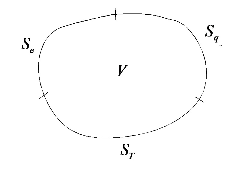
As shown in Figure 9.1, the object subject to thermal analysis consists of a domain \(V\) and a boundary \(S\). The boundary \(S\) is divided into the boundary \(S_q\) where the heat transfer rate is prescribed, the boundary \(S_T\) where the temperature is prescribed, the boundary \(S_e\) where radiative and convective heat transfer occur, the die-workpiece contact surface \(S_c\), and so on. A certain amount of the energy applied to the workpiece (the stress power \(\sigma_{ij}\dot{\varepsilon}_{ij}\)) is released as plastic heat, and the remainder is regarded as being stored as internal energy; the frictional work generated at the contact surface is regarded as being transferred to the die and the workpiece at (0–50)% each. The thermal conductivity, specific heat, and so on are given as functions of temperature.
9.2 Finite Element Formulation
The heat transfer phenomenon in a solid is formulated by the following heat conduction equation for a solid.
Here \(T\) and \(t\) denote the temperature and time, respectively, and \(k\) and \(\rho c\) denote the thermal conductivity and the heat capacity, respectively, and are functions of the coordinates and the temperature. \(Q\) is the heat generation rate, consisting of the heat generation rate due to deformation energy and the heat generation rate \(Q_0\) due to other heat sources. That is, the heat generation rate is expressed as
The heat generation ratio coefficient \(C_g\) denotes the proportion of the stress power \(\sigma_{ij} \dot{\varepsilon}_{ij}\) that is converted into heat. In general, it is known that about 90% (\(C_g = 0.9\)) of the stress power is converted into plastic heat, and the remainder is consumed by increases in internal energy such as changes in the crystal structure of the material, residual deformation energy, and the increase of dislocations.
The aforementioned boundary conditions are formulated as follows.
Here \(n_i\) is the outward unit normal vector, and \(\bar{T}\), \(T_c\), \(T_w\), \(T_e\) denote the prescribed temperature, the surface temperature of the contacting body, the temperature of the coolant, and the ambient temperature, respectively, and \(h_c\), \(h_q\), \(h_e\) denote the heat transfer coefficient at the contact surface, the convective heat transfer coefficient with the coolant, and the convective heat transfer coefficient with the surrounding environment, respectively. \(\sigma\varepsilon\) is the product of the Stefan-Boltzmann constant and the emissivity of the body. \(q_f\) denotes the heat generation rate produced at the contact surface by friction, and is given as follows.
Here \(v_t\) and \(\bar{v}_t\) are the tangential velocity components of the workpiece and the die, respectively, and \(\sigma_t\) is the tangential stress at the contact surface. \(C_f\) is a constant taking a value between 0.0 and 0.5, and is intended to account for the frictional heat at the interface.
The weak form of the above boundary value problem is as follows.
The detailed derivation process and solution method of the finite element equations are left to reference [1.1].
9.3 Coupled Analysis
Plastic heat is generated in both cold and hot metal-forming processes. In general, the plastic heat in cold forming causes a temperature rise in the workpiece and the die, but it is known that the change in flow stress due to the raised temperature is small. On the other hand, in hot metal forming, the generation of plastic heat and the temperature change due to heat transfer between the workpiece and the die directly affect the flow stress of the workpiece. That is, in Equation (8.3) of the flow analysis problem, \(\bar{\sigma}\) is a function of temperature, and in Equation (9.1) of the thermal analysis problem, \(Q\) is a function of the strain rate or the velocity field.
Therefore, since the flow analysis problem and the thermal analysis problem are coupled, this is called a coupled problem, and analyzing and characterizing the coupled problem is called coupled analysis or non-isothermal analysis. It is practically impossible to solve the coupled problem by directly assembling it into a simultaneous system or by eliminating variables. This is because, although the actual object of analysis, the workpiece, is a single body, there are at least two dies (including the punch); when there are two dies, there are three thermal analysis problems and one flow analysis problem, so the numerical computation is practically impossible.
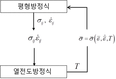
To resolve this problem, a staggered iterative convergence technique for the thermal analysis–flow analysis problem, as shown in Figure 9.2, is generally used. The thermal analysis problem and the flow analysis problem are separated and solved independently, but in the thermal analysis the stress power (\(\sigma_{ij}\dot{\varepsilon}_{ij}\)), which is the result of the flow analysis, is used, and the temperature information needed in the flow analysis is taken from the result of the thermal analysis. During the thermal analysis the flow field does not change, and during the flow analysis the temperature field does not change. If this numerical analysis process is repeated, the changes in the flow field and the temperature field simultaneously and gradually decrease, and finally a converged solution is reached.
Coupled analysis requires the thermal information of the workpiece and thermal boundary-condition information. The simulation results are greatly influenced by such thermal information. Many researchers are studying this through experiment and analysis, but users still have access only to limited information. Therefore, users' own efforts to obtain the necessary thermal information must be continued. Meanwhile, in actual process-application studies, isothermal analysis is mostly performed. Isothermal analysis is a term referring to performing a simulation under the assumption that there is no temperature change during the process. In this case, the material properties of the workpiece can be obtained from the average temperature of the workpiece. Such workpiece information can be obtained relatively easily. Empirically, even when isothermal analysis is performed, the metal flow lines and so on can be predicted accurately.
Isothermal analysis refers to a plastic flow analysis under the assumption that the temperature is constant by neglecting the effect of temperature. Forging performed while maintaining a constant temperature for the production of parts with extremely poor forgeability or special parts is called isothermal forging; isothermal analysis should not be associated with isothermal forging.
9.4 Approximate Solution Method for Temperature
In metal-forming simulation from a macroscopic viewpoint, the analysis of temperature is sometimes important, but empirically, in the flow analysis of most general metal-forming processes, temperature is not a major variable. Even if temperature is important, there are many constraints on improving the reliability of the temperature prediction results. First, the heat transfer phenomenon at the moment of contact between the workpiece and the die in metal forming is close to a thermal shock. In order to accurately predict such a phenomenon by numerical methods, a very dense mesh in the depth direction of the die and the workpiece must be supported, but this is not realistic because it causes a sharp increase in the computation time not only for the heat transfer analysis but also for the plastic flow analysis.
Second, even if there is no methodological deficiency, accurately modeling the boundary conditions is not an easy task. If a large cost is invested, it is possible to obtain better information, but what is gained from this is less than expected. Therefore, the rate of improvement of such thermal information is likely to remain below expectations.
In general hot forging processes, it is not common for the workpiece to separate from the die after it has come into contact with it. And after the workpiece comes into contact with the die, the decrease in the surface temperature of the workpiece and the rise in the surface temperature of the die can be assumed to be in a functional relationship to some extent. Of course, if this functional relationship can be clearly known, non-isothermal analysis from the workpiece viewpoint would become advantageous.
Taking this into account, an approximate non-isothermal metal-forming process analysis function based on a die-temperature prediction method that considers the temperature history of the workpiece in contact with the die has been developed [9.1].
In general, non-isothermal analysis is based on the convergence of two problems: the convergence of the thermal analysis and flow analysis problems of the workpiece, and the convergence of the thermal analysis problems of the workpiece and the die. Therefore, obtaining a rigorously converged solution inevitably takes a great deal of time. Of course, for the purpose of computing an engineering solution, the number of iterations is sometimes limited.
An approximate solution method that estimates the die temperature instead of performing thermal analysis of the die, that is, a workpiece-centered non-isothermal analysis technique, can have advantages. Of course, in this technique, not only the actual temperature of the workpiece but also the approximately computed die-temperature information is stored as nodal values of the workpiece. At each analysis step, based on the change \(\Delta T_m^i\) in the actual temperature of the workpiece at the contact surface, an approximate value \(\Delta T_d^i\) of the die-temperature change is computed as follows.
Here \(\alpha\) is a constant based on empirical values, and the '−' in Equation (9.10) means that the die temperature rises as the workpiece cools. In order to evaluate the aforementioned technique, the proposed technique was applied to an axisymmetric process. The main information of the process is as follows. Workpiece type: SCr420HB; die type: SKD61; initial workpiece size: (diameter) 8.0, (height) 12.0 mm; initial workpiece temperature: 1100°C; initial die temperature: 150°C; friction law: Coulomb friction law (Coulomb friction coefficient, \(\mu=0.2\)).

(a) Workpiece

(b) Die
Figure 9.3 Comparison of two-dimensional and three-dimensional non-isothermal prediction results
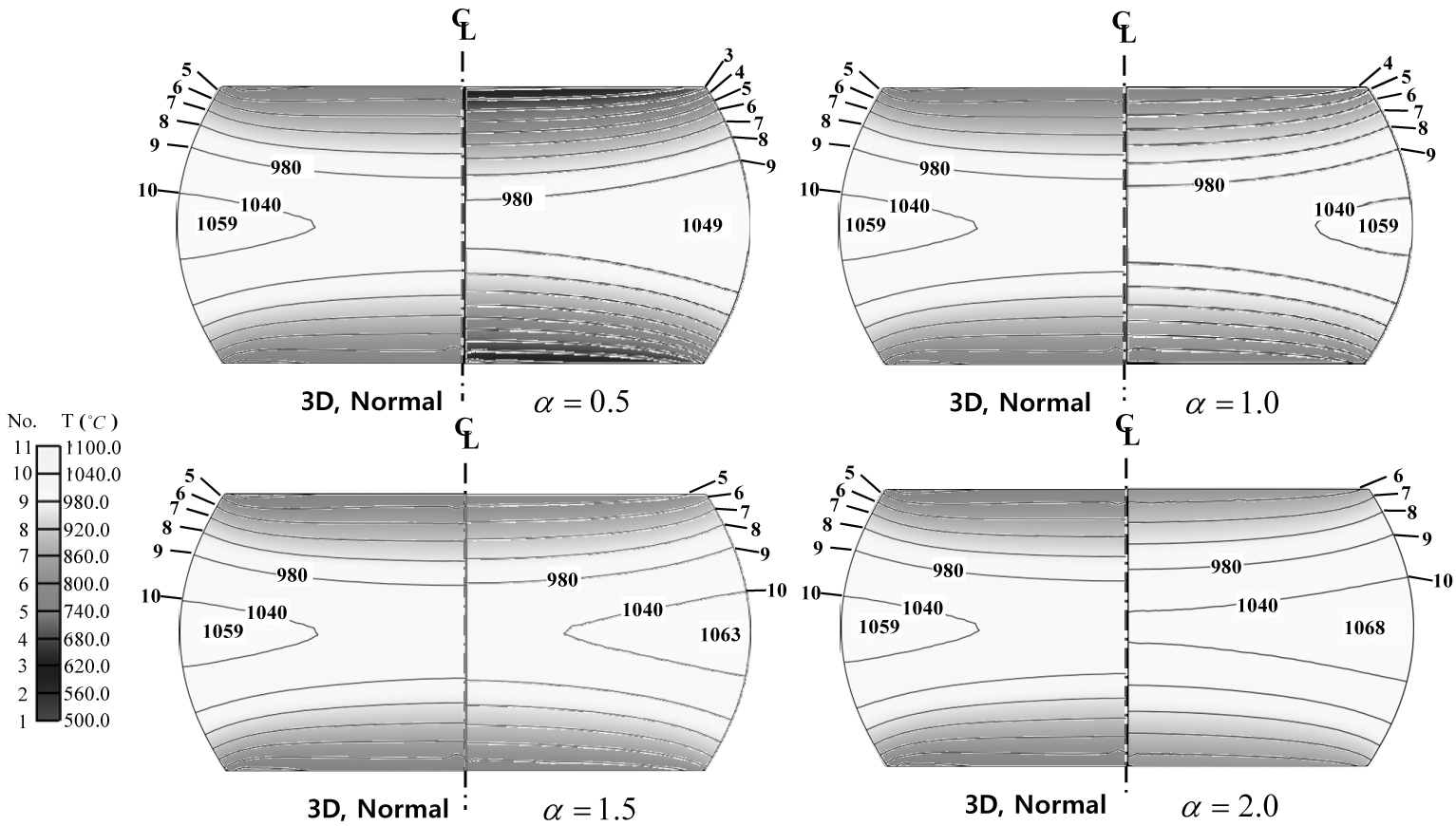
First, let us examine the temperature distribution of the workpiece in Figure 9.3(a) obtained by the standard method. In the two-dimensional analysis result, the maximum and minimum temperatures are 1061.0℃ and 743.0℃, respectively, and in the three-dimensional analysis result, the maximum and minimum temperatures are 1059.0℃ and 733.0℃, respectively. Therefore, the difference is not large from an engineering standpoint, and it is negligible when the differences in the theoretical background and approach between two and three dimensions and the effect of the mesh are taken into account. The die-temperature distribution in Figure 9.3(b) is likewise the same.
Figure 9.4 was obtained by applying the approximate non-isothermal analysis technique, and it can be seen that for \(\alpha=1.0\) and \(\alpha=1.5\) there is no large difference from the standard solution. On the other hand, the approximate solutions predicted by \(\alpha=0.5\) and \(\alpha=2.0\) differ somewhat from the standard solution.