6 Damage and Ductile Fracture Theory

6.1 Traditional Ductile Fracture Theory

The reason a material reaches fracture differs from material to material. For this reason, a variety of fracture theories suited to the characteristics of each material have been developed. At present, the theory that is persuasive from the standpoint of metal forming is ductile fracture theory. In this theory, fracture occurs when the value of the damage accumulated in the material reaches the limit value that the material can withstand, that is, the critical damage. Therefore, to use this theory effectively, the selection of a damage model suited to the material and the determination of an appropriate critical damage must be presupposed. Empirically, the predicted damage results vary somewhat depending on the choice of the damage model. Damage models studied to date for the purpose of fracture analysis include energy-based models (Cockroft and Latham, Freudenthal), void-growth micromechanics-based damage models (McClintock, Rice and Tracey, Oyane), porous-material-based models (Tvegaard and Needleman), and continuum-damage-mechanics-based damage models (Lemaitre). The damage models most commonly used are summarized below.

ⓐ Normalized Cockcroft-Latham damage model

\[ D = \int_0^{\bar{\varepsilon}_f} \frac{\langle \sigma_1 \rangle}{\bar{\sigma}} d\bar{\varepsilon} \tag{6.1} \]

ⓑ Cockcroft-Latham damage model

\[ D = \int_0^{\bar{\varepsilon}_f} \sigma_1 d\bar{\varepsilon} \tag{6.2} \]

ⓒ Brozzo, Deluca, Rendina damage model

\[ D = \frac{2}{3} \int_0^{\bar{\varepsilon}_f} \frac{\sigma_1}{\sigma_1 + p} d\bar{\varepsilon} \tag{6.3} \]

ⓓ Freudenthal damage model

\[ D = \int_0^{\bar{\varepsilon}_f} \bar{\sigma} d\bar{\varepsilon} \tag{6.4} \]

ⓔ McClintock damage model

\[ D = \frac{1}{2} \int_0^{\bar{\varepsilon}_f} \left[ \frac{2}{\sqrt{3}(1-n)} \sinh \left[ \frac{\sqrt{3}}{2}(1-n) \frac{\sigma_1 + \sigma_3}{\bar{\sigma}} \right] - \frac{\sigma_3 - \sigma_1}{\bar{\sigma}} \right] d\bar{\varepsilon} \tag{6.5} \]

ⓕ Oyane, Okimoto, Shima damage model

\[ D = \int_0^{\bar{\varepsilon}_f} \left( 1 - \frac{p}{A\bar{\sigma}} \right) d\bar{\varepsilon} \tag{6.6} \]

ⓖ Norris, Reaugh, Moran, Quinnones damage model

\[ D = \int_0^{\bar{\varepsilon}_f} \frac{\bar{\sigma}}{1+cp} d\bar{\varepsilon} \tag{6.7} \]

ⓗ Rice-Tracey damage model

\[ D = \int_0^{\bar{\varepsilon}_f} A \exp \left( \frac{3}{2} \frac{\sigma_m}{\bar{\sigma}} \right) d\bar{\varepsilon} \tag{6.8} \]

In the equations above, \(\sigma_1 \ge \sigma_2 \ge \sigma_3\) are the principal stresses, and \(p = -\sigma_m\) is the hydrostatic pressure. Also, \(c\), \(A\), and \(n\) are material constants. \(\langle x \rangle\) is the Macaulay (singularity) function, which takes the value \(0\) when \(x\) is negative and the value \(x\) when \(x\) is positive. In the McClintock damage model, the damage when \(n=1.0\) is identical to the damage of the normalized Cockcroft-Latham damage model.

6.2 Triaxial-Stress-Based Damage Model

6.2.1 Shear Fracture During Metal Forming

Owing to recent lightweighting issues, the strength of metal sheets is steadily increasing. When forming high-strength metal sheets, problems such as insufficient formability of the material, breakage of the die, control of springback, and shear fracture are continually being raised, and much research is being carried out. Among these, shear fracture occurs in the sheet forming of high-strength steel sheets when the shoulder radius of the die is excessively small relative to the sheet thickness; in the narrow region of the material-die contact, fracture occurs due to the local concentration of strain resulting from excessive bending. This is reported to occur because of the relatively lower ductility of high-strength steel compared with mild steel. Figure 6.1 shows an example of shear fracture that occurs in an actual high-strength steel sheet. Many prior studies have investigated the shear fracture of high-strength steel sheets.

Figure 6.1 Example of shear fracture in the metal forming of a high-strength steel sheet [6.1]

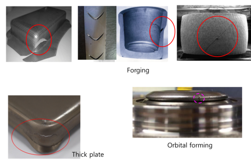
Such a fracture strain lies in a shear-deformation region that cannot be predicted in the FLD (Forming Limit Diagram) plane, which is composed of major-direction and minor-direction strains. This is referred to as in-plane shear deformation. Therefore, a new fracture model that includes not only uniaxial tension and biaxial tension but also the shear-deformation region is needed, and Li et al. [6.2] showed that fracture prediction is possible using the modified Mohr-Coulomb model [6.3]. From here on, the triaxial-stress fracture theory that applies the recent research results of Bai and Wierzbicki [6.4] is described in a limited manner.

6.2.2 Damage Model Theory Under Triaxial Stress States

(1) Acquisition of material properties from the tensile test

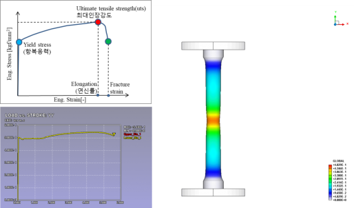
As shown in Figure 6.2, in the case of one-dimensional fracture prediction, the fracture of the material occurring during metal forming is predicted based on the strain at the endpoint of the maximum uniform elongation interval obtained from the tensile test, that is, the strain at the necking point or the fracture point, i.e., the fracture strain. At this time, the maximum stress or the maximum strain is taken as the fracture criterion. Such a one-dimensional fracture prediction technique based on the tensile test is not suitable for sheet forming, which passes through complex stress states.

Figure 6.2 Tensile test and fracture curve

To overcome the limitations of such tensile-test-based fracture prediction theory, the fracture limit for each fixed strain path was introduced as a limit curve for sheet forming, and this curve is called the forming limit curve, that is, the FLD (Forming Limit Curve). The forming limit curve of Figure 6.3 is used as a very valid basis for fracture within the range of the deformation paths (uniaxial tension-plane-strain tension-biaxial tension) mainly experienced in the drawing process among the types of sheet forming. However, as shown in Figure 6.3, the fracture strain cannot be measured for the shear region or for compressive stresses. Furthermore, because a fixed stress ratio is assumed, it is valid only for a fixed metal forming path. Therefore, it is not valid for complex drawing processes, or for processes in which the deformation path changes, including ironing tension-compression processes.

To resolve such problems, research on the TFD (Triaxiality Failure Diagram), which considers the triaxial stress state, has recently been actively conducted. In the case of the TFD, the analysis of the fracture phenomenon is carried out in the local region where fracture deformation occurs for specimens of various stress states. Because it is not a theoretical formulation that assumes a fixed strain path, it has the advantage of not being dependent on the deformation path.

To measure the local fracture elongation needed to construct the TFD, the DIC (Digital Image Correlation) technique is used, in which a special paint is applied to the surface of the metal specimen and the displacement of the paint particles is photographed to compute the strain. In this method, the fracture strain is determined through tuning with a finite element analysis model for calibration. Therefore, it has the disadvantage of taking a long time owing to the excessive measurement time and the determination of numerous finite element analyses and variables.

Figure 6.3 Forming limit curve (FLD) and FLD test specimen

Figure 6.4 DIC measurement system linked with a universal tensile testing machine

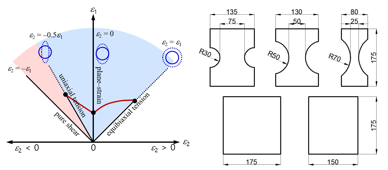
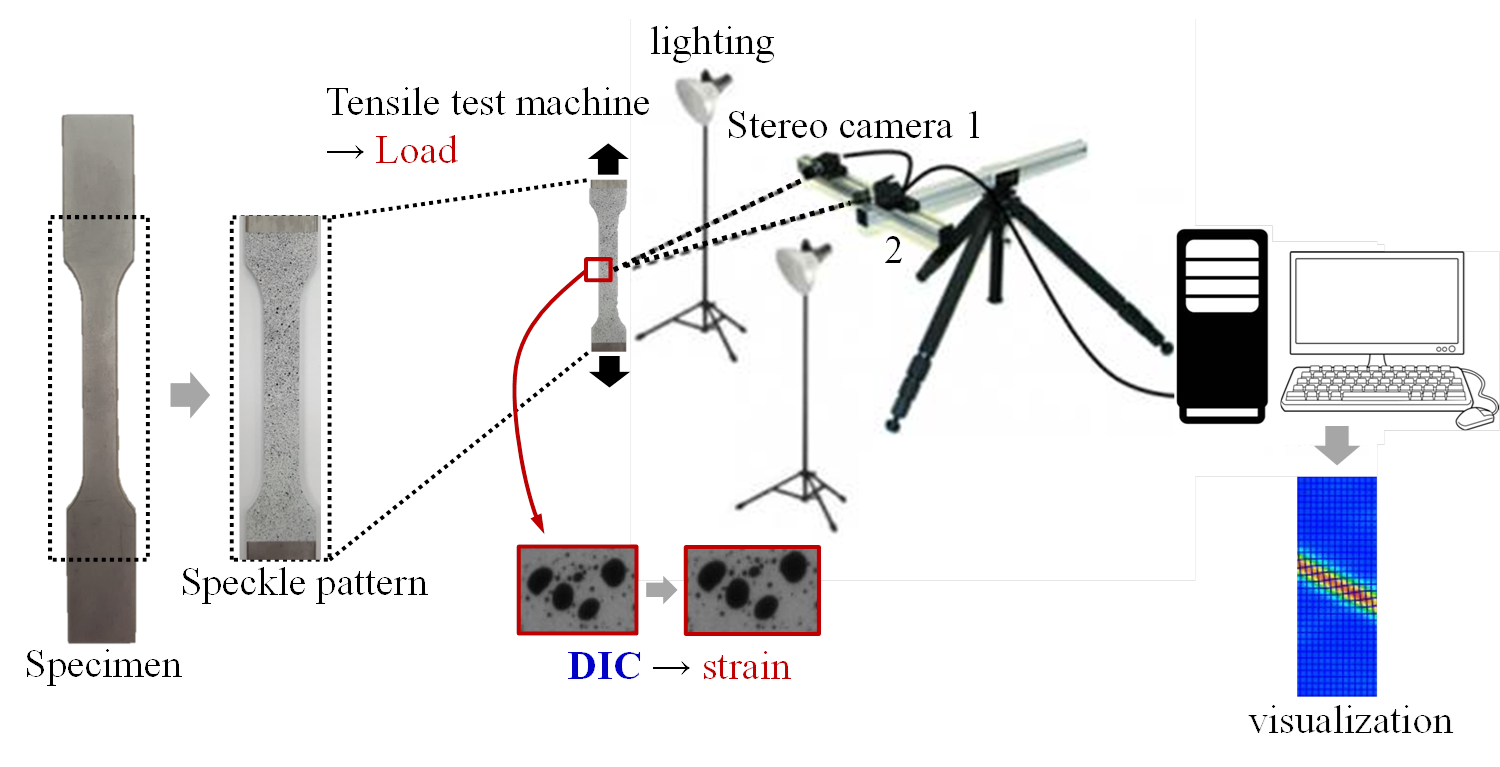
Figure 6.4 introduces the DIC measurement equipment and method. After applying a special spray onto the metal specimen to generate an irregular pattern, the displacement of the pattern is photographed by two stereo cameras during the tensile test, and the strain distribution is computed after the tensile test is completed. Because the strain distribution over the entire measured region can be computed, it has the advantage that even the fracture strain of the local region can be measured.

Figure 6.5 shows the strain distribution at the moment of fracture measured by DIC for a tensile specimen of Al6061 alloy. This figure shows that, whereas the magnitude of strain obtainable through an ordinary tensile test is the strain up to the uniform elongation at which necking occurs, that is, about 15%, when DIC is used the strain can be measured until the local elongation reaches a maximum of 60%. Therefore, the local fracture strain of each stress state can be measured or tracked, and the fracture strain for each stress state can be measured through DIC tensile tests of various shapes.

Figure 6.5 Strain distribution over the entire region obtained using DIC in the tensile test

Figure 6.6 TFD (Triaxiality Failure Diagram)

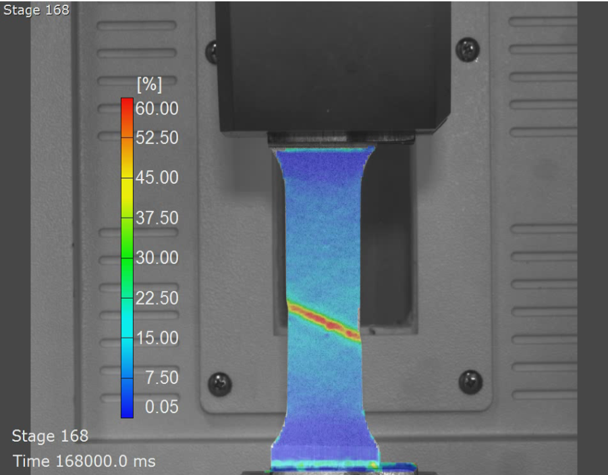
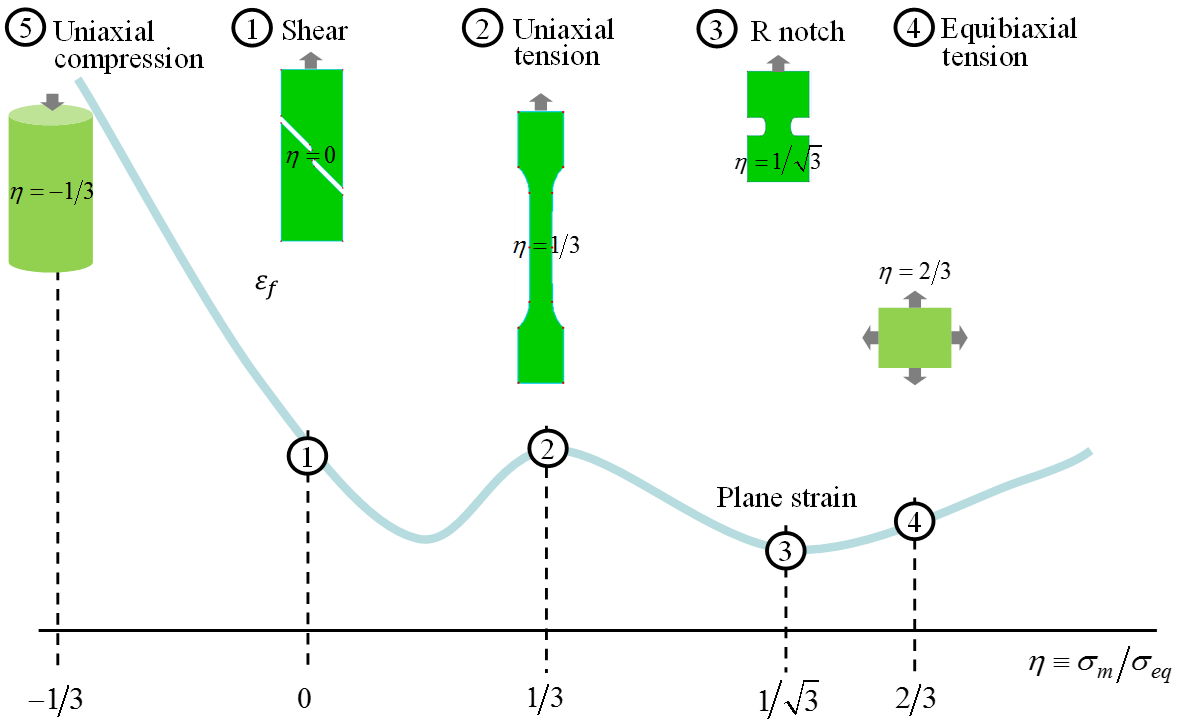
Figure 6.6 shows a conceptual diagram of the TFD. In the figure, the curves show the fracture strain together with the specimen shapes for each stress state used in sheet forming, that is, (1) shear, (2) uniaxial tension, (3) plane strain, and (4) biaxial tension. The \(x\)-axis of the TFD is expressed as a small real value, defined by the stress triaxiality factor \(\eta\) (the ratio of \(\sigma_m\), the mean stress, to \(\bar{\sigma}\), the effective stress); the stress triaxiality factor based on the effective stress is defined by the following equation.

\[ \eta = \frac{\sigma_m}{\bar{\sigma}} \tag{6.9} \]

Here, \(\sigma_m\) denotes the mean stress and \(\bar{\sigma}\) denotes the effective stress. This stress triaxiality factor, together with the Lode angle (see Equation (6.21)), is a representative stress-based variable that indicates the loading path. Whereas the FLD used in sheet forming is a strain-based fracture limit diagram and has restrictions on the deformation path, the fracture limit diagram using stress triaxiality (TFD) has the characteristic of being independent of the deformation path.

The effective stress corresponding to the von Mises yield theory that considers three-dimensional stress is given by the following equation.

\[ \bar{\sigma} = \sqrt{\frac{1}{2} \left[ (\sigma_1 - \sigma_2)^2 + (\sigma_2 - \sigma_3)^2 + (\sigma_3 - \sigma_1)^2 \right]} \tag{6.10} \]

For sheet forming problems, a plane stress state with a two-dimensional constitutive model is assumed. That is, because only \(\sigma_1\) and \(\sigma_2\) are considered and the through-thickness stress \(\sigma_3\) of the sheet is assumed to be \(0\), Equation (6.10) is expressed by the following concise equation.

\[ \bar{\sigma} = \sqrt{\sigma_1^2 + \sigma_2^2 - \sigma_1\sigma_2} \tag{6.11} \]

The specimen shapes of Figure 6.6 were determined from finite element analysis so that each stress state proceeds. Because thin sheet metal is in a plane stress state (\(\sigma_3 = 0\)), the representative stress states can be easily computed. For the shear specimen, \(\eta = 0\) (\(\sigma_1 = \sigma_2 = 0\)); for the uniaxial tension specimen, \(\eta = 1/3\) (\(\sigma_1 = \bar{\sigma}, \sigma_2 = \sigma_3 = 0\)); and for biaxial tension, \(\eta = 0.66\) (\(\sigma_1 = \sigma_2 = \bar{\sigma}\)).

The GISSMO (Generalized Incremental Stress State damage MOdel), developed by Neukamm et al. [6.5, 6.6], is a phenomenological formulation for ductile damage that describes the instability, softening, and fracture of a material. The decrease in stress after a certain interval is expressed as the material having sustained damage; damage begins from the moment the plastic deformation of the material starts, gradually accumulates, and, upon reaching the critical value, fracture occurs. \(D = 0\) corresponds to undeformed material, and \(D = 1\) becomes the criterion for measuring fracture. The damage accumulation is based on the following.

\[ \Delta D = \frac{n_D}{\bar{\varepsilon}_f} D^{(1 - \frac{1}{n_D})} \Delta \varepsilon_p \tag{6.12} \]

Here, \(D\) is the damage and \(n_D\) is the damage exponent. \(\bar{\varepsilon}_f\) is the effective strain at fracture, and \(\Delta \varepsilon_p\) is the effective plastic strain increment. The experimental values obtained by the DIC (Digital Image Correlation) technique in the tensile test are set as the initial input values, and optimization is performed so that the force-displacement values predicted through the finite element analysis program become equal to the experimental values, thereby determining the coefficients of Equation (6.12).

(2) Finite element modeling of the triaxial-stress fracture curve

By applying a constitutive equation that couples the flow stress and the damage, a softening technique that causes an artificial reduction of the flow stress after the maximum tensile load (necking strain), as well as techniques such as mesh deletion, are included in the finite element modeling. Equation (6.13), the coupling of plasticity and the damage model, shows the fracture behavior.

\[ \sigma^* = \bar{\sigma} (1 - \Delta D)^m \tag{6.13} \]

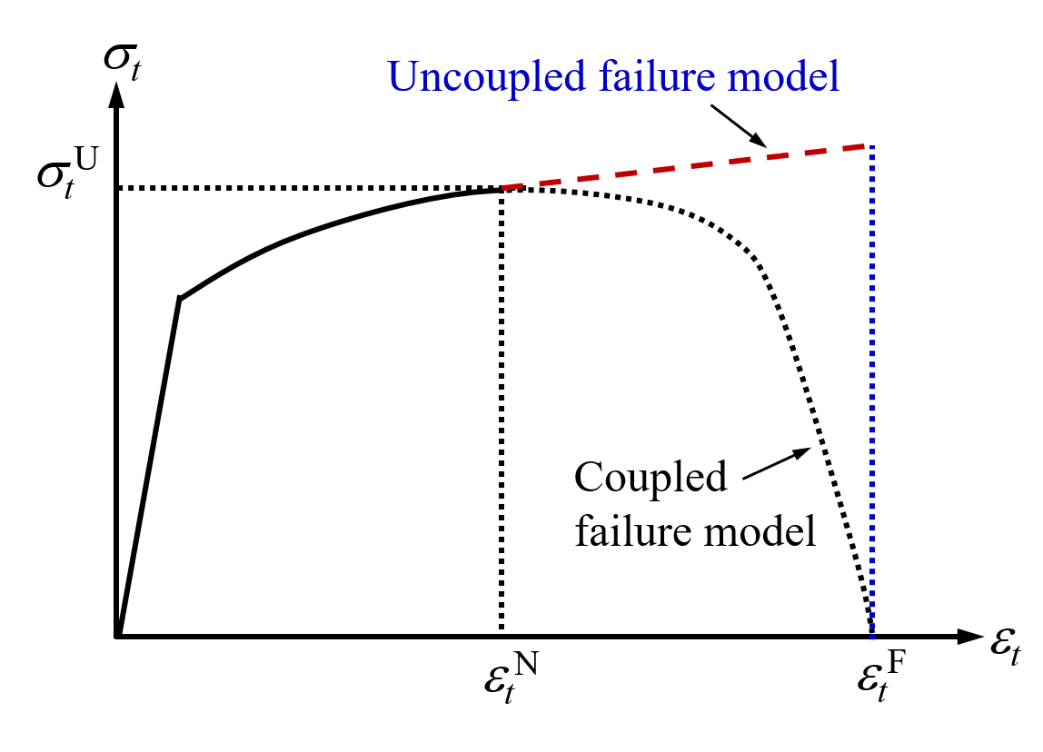
Here, \(\sigma^*\) and \(\bar{\sigma}\) denote the softened flow stress and the reference effective stress, respectively, and \(m\) is the fading exponent that leads to material fracture and is a kind of material constant. Therefore, as shown in Figure 6.7, an accurate representation of the damage behavior after necking is possible. In Figure 6.7, \(\sigma_t^U\) denotes the true stress corresponding to the tensile strength, and \(\varepsilon_t^N\) and \(\varepsilon_t^F\) denote the true strain at the necking point and the maximum true strain at the fracture point, respectively.

Figure 6.7 Deformation characteristics for the damage and fracture models

(3) Tensile test and DIC test

The tensile test must be performed under quasi-static loading conditions in different stress states, and the most commonly used equipment for the tensile test is the universal testing machine or the tensile tester. The machine has two crossheads, one used to adjust the length of the specimen and the other used to constrain the specimen.

Strain gauges attached to the surface of the specimen and non-contact optical extensometers are used to measure the dynamic strain or displacement. The inertia of the strain gauge and the extensometer affects the experimental results. Therefore, to safeguard the quality of the displacement and strain measurement results, careful attention must be paid to the use of the equipment. To obtain the accurate trajectory of the crack, the use of the scientific method by DIC is preferable to visual inspection. Using DIC, reliable data on the time-dependent displacement and deformation over the entire measurement region can be obtained from the tensile test.

(4) Bai-Wierzbicki model

One of the models for which much applied research has recently been carried out is the Bai and Wierzbicki (BnW) model. Using the stress triaxiality factor (\(\eta\)) and the Lode angle (\(\theta\)) or the normalized Lode angle (\(\bar{\theta}\)), they proposed a damage model based on fracture theory, that is, ductile fracture theory, and it showed good agreement with experimental results [6.4].

The damage \(D\), which serves as the measure of fracture, is defined as follows.

\[ D = \sum_i \frac{\Delta \bar{\varepsilon}_p^i}{\bar{\varepsilon}_p^{crit}} \tag{6.14} \]

Here, \(\bar{\varepsilon}_p^i\) is the plastic strain increment at the \(i\)-th analysis step. \(\bar{\varepsilon}_p^{crit}\) is defined as the BnW fracture strain and is defined as a function of the stress triaxiality factor \(\eta\) and the angle to the principal direction, that is, the Lode angle \(\theta\) or the normalized Lode angle \(\bar{\theta}\), as follows.

\[ \bar{\varepsilon}_p^{crit} = f(\eta, \theta) \tag{6.15} \]

or

\[ \bar{\varepsilon}_p^{crit} = f(\eta, \bar{\theta}) \tag{6.16} \]

Here, the stress triaxiality factor \(\eta\) is defined as follows,

\[ \eta = \frac{\sigma_m}{\bar{\sigma}} = \frac{\sigma_1 + \sigma_2 + \sigma_3}{3\bar{\sigma}} \tag{6.17} \]

and the Lode angle \(\theta\) and the normalized Lode angle \(\bar{\theta}\) are defined by the following equations, respectively.

\[ \theta = 2\frac{\sigma_2 - \sigma_3}{\sigma_1 - \sigma_3} - 1 \tag{6.18} \]

\[ \bar{\theta} = 1 - \frac{2}{\pi} \cos^{-1} \left( \frac{r}{\bar{\sigma}} \right)^3 \tag{6.19} \]

where \(r\) is

\[ r = \left[ \frac{27}{2} (\sigma_1 - \sigma_m)(\sigma_2 - \sigma_m)(\sigma_3 - \sigma_m) \right]^{\frac{1}{3}} \tag{6.20} \]

which is a function of the third invariant of the deviatoric stress tensor. The plastic strain increment (\(\Delta \bar{\varepsilon}_p^i\)) is computed from the product of the strain rate (\(\dot{\bar{\varepsilon}}\)) and the time increment of the analysis step (\(\Delta t\)).

The BnW fracture strain \(\bar{\varepsilon}_p^{crit}\) based on the normalized Lode angle is computed by the following equation.

\[ \bar{\varepsilon}_p^{crit} = C1 + C2 + C3 \tag{6.21} \]

\[ \begin{aligned} C1 &= \left[ 0.5 (D_1 e^{-D_2 \eta} + D_5 e^{-D_6 \eta}) - D_3 e^{-D_4 \eta} \right] \bar{\theta}^2 \\ C2 &= \left[ 0.5 (D_1 e^{-D_2 \eta} - D_5 e^{-D_6 \eta}) \right] \bar{\theta} \\ C3 &= D_3 e^{-D_4 \eta} \end{aligned} \tag{6.22} \]

Here, \(D_1, D_2, D_3, D_4, D_5\), and \(D_6\) are material constants, called the coefficients of the Bai-Wierzbicki model. If the normalized Lode angle \(\bar{\theta}\) is replaced by the Lode angle \(\theta\), these coefficients may also change slightly. In general, since the Bai-Wierzbicki model based on the normalized Lode angle is mainly used, coefficients used without special mention are understood to be based on the normalized Lode angle \(\bar{\theta}\).

Bai and Wierzbicki performed fracture tests of various stress states on Al-2004-T5 material. Table 1 summarizes the coefficients of the Bai-Wierzbicki model for Al-2004-T5.

[Table 6-1] Coefficients of the Bai-Wierzbicki model

D1	D2	D3	D4	D5	D6
0.063112	-4.94622	0.212041	-1.5111	0.21626	3.72498

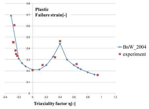
Figure 6.8 shows a comparison graph of the experimental fracture limit of Al2004-T5 and the Bai-Wierzbicki model.

Figure 6.8 Comparison of the fracture test and the BnW 2004 model

To aid understanding, let us compute the triaxial stress state. Figure 6.9 defines the problem for the computation of the triaxial stress state in this section and the computation of the damage in the next section. This process is a thick-plate burring process, which has the characteristic of being sensitive to fracture. The material is Al-2004-T5, and the friction coefficient is assumed to be 0.05.

Figure 6.9 Definition of the problem for the computation of the triaxial stress state and the damage

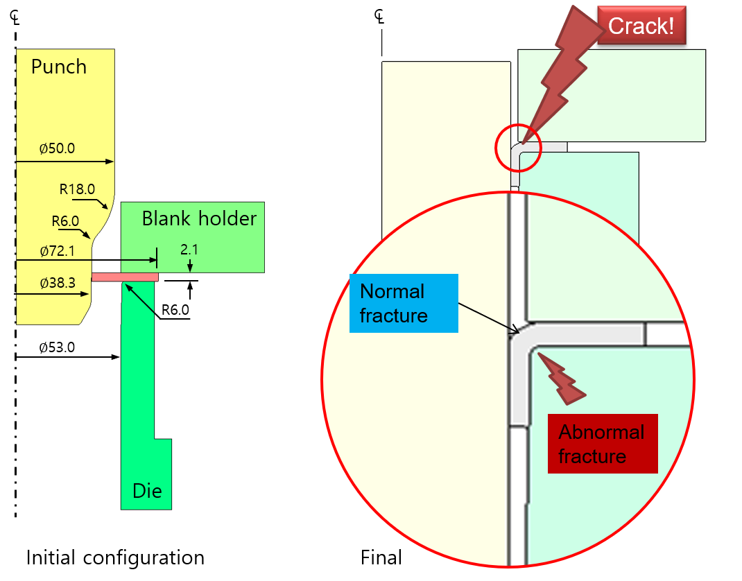
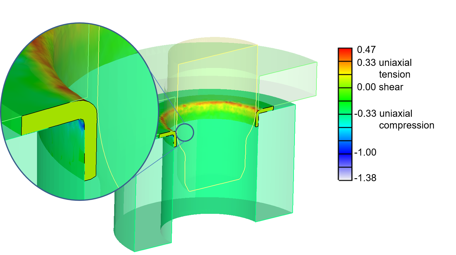
Figure 6.10 shows the distribution of the triaxial stress state. It can be confirmed that the \(\eta\) value changes greatly at the outer and inner surfaces of the corner.

Figure 6.10 Stress triaxiality factor

6.3 Comparison of Damage Models

In this section, the damage models introduced above are compared. For the same process used in the previous section, various damage models were applied and the results are presented across Figures 6.11-6.16.

Figures 6.11, 6.12, and 6.15 are similar, and the accumulation of damage is prominent near the inner corner. This is because, as can be seen from the Cockcroft-Latham model equation, the three related damage models depend on the influence of the maximum principal stress (which is mostly tensile stress). This can be seen directly from Equations (6.1), (6.2), and (6.3), and the characteristics of these damage models can be seen indirectly from the fact that the McClintock model with \(n = 1.0\) is almost identical to the normalized Cockroft-Latham model. As shown in Figure 6.9, this model is suitable for predicting the normal fracture of the convex corner generated during the deburring process. However, it cannot predict the fracture of the concave corner, which uncommonly occurs depending on the material. On the other hand, although the variable \(n\) in the McClintock model is a value between \(0.0\) and \(1.0\), the difference in the results for this example according to this value is not very large. Figure 6.12 is the case of \(n = 0.0\); there is a tendency for the distribution to spread as the value of \(n\) increases, but the change is not large.

Figure 6.11 Normalized Cockcroft-Latham damage model Figure 6.12 McClintock (=0.0) damage model

The Rice-Tracy model of Figure 6.13 also shows a tendency similar to these. This is because, due to the form of the integrand of the assumed natural exponential function, the influence of the tensile stress is inevitably overestimated relative to the others. On the other hand, the Oyane et al. model and the Bai-Wierzbicki model predict similar damage distributions. As can be seen in Equation (6.6), the Oyane model is fundamentally also dependent on the mean stress, but it is characterized by adding strain to the damage and by causing a decrease in damage when the mean stress is negative. Therefore, it is highly likely to predict high damage at the concave corner where the strain is large. Therefore, as shown in Figure 6.9, it can be used for the purpose of predicting the crack that occurs at the corner.

Figure 6.11 Normalized Cockcroft-Latham damage model Figure 6.12 McClintock (=0.0) damage model

Because the Bai-Wierzbicki model is mathematically complex, it is not easy to assign a physical meaning from the equations compared with other models. However, as shown in Figure 6.6, it has the advantage of being able to represent various theoretically clear cases according to the stress triaxiality factor.

Figure 6.11 Normalized Cockcroft-Latham damage model Figure 6.12 McClintock (=0.0) damage model

6.4 Damage-Coupled Flow Stress

Even if the softening phenomenon due to the accumulation of damage is not reflected in the analysis process, the damage can be usefully employed to determine whether fracture occurs. For this reason, the damage-dependent softening phenomenon is not considered in actual industrial practice. If this softening phenomenon is not considered, that is, if the damage and the flow stress are not coupled, the damage model does not affect other prediction results, including the forming load and the deformation.

Conversely, if the damage and the flow stress are coupled, it may have some influence on the overall analysis results. If material-science phenomena are to be reflected, the method of coupling can be complex. For example, the dislocation density and the like may be used as parameters. However, to obtain an engineering solution, a simple function can be useful according to the purpose of phenomenological observation and prediction. That is, a function for softening, namely a room-temperature flow-stress softening function \(\delta(D)\), can be used in addition to the existing flow stress function as follows.

\[ \bar{\sigma} = Y_0(1 + \bar{\varepsilon}/b)^n \delta(D) \tag{6.23} \]

Figure 6.17 Example of a room-temperature flow-stress softening function

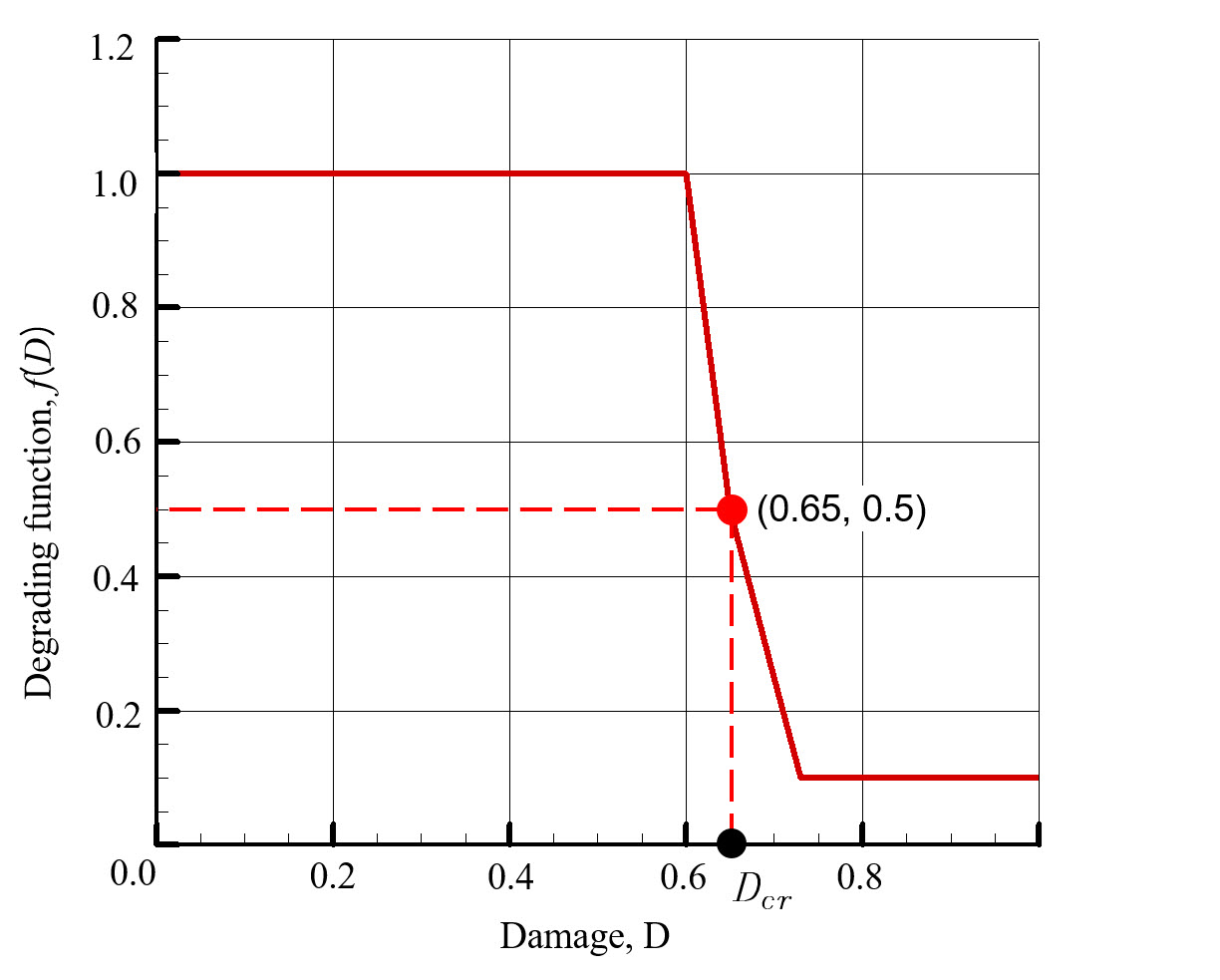
In Equation (6.13), the exponential function, one of the forms of \(\delta(D)\), has already been introduced. Figure 6.17 is an example of \(\delta(D)\) expressed as a piecewise-linear function of the damage. This function is a room-temperature flow-stress softening function that, when the damage reaches the critical damage, forcibly reduces the flow stress by the ratio of \(\delta(D)\).

Figure 6.18 shows the deep-piercing fracture analysis results using the element-degradation technique with the room-temperature flow-stress softening function of Figure 6.17 and the damage-based crack propagation technique. A point to note in the analysis of this process is that, owing to the process characteristics of deep piercing, applying the crack propagation technique from the beginning causes many numerical difficulties.

(a) Element-degradation technique (flow stress distribution)

(b) Fracture analysis by crack propagation

Figure 6.18 Analysis of the deep-piercing process using the element-degradation technique